Wannierization

Often we only care about a few bands, for example the bands near the Fermi energy. Wannierization builds a smaller tight-binding model that describes only these bands. We do this with h.get_wannier_hamiltonian().

Maximally localized Wannier functions

Take a group of \(J\) bands that is separated from the other bands by a gap in the whole Brillouin zone. From their Bloch states \(|\psi_{mk}\rangle\) we build localized orbitals, the Wannier functions,

\[ |w_{n\mathbf R}\rangle = \frac{1}{N_k}\sum_{\mathbf k} e^{-i\mathbf k\cdot\mathbf R} \sum_{m=1}^{J} U_{mn}(\mathbf k)\,|\psi_{m\mathbf k}\rangle , \]

where \(\mathbf R\) is a unit cell, \(N_k\) is the number of k-points of the mesh, and \(U(\mathbf k)\) is a unitary \(J\times J\) matrix at each k-point. The Bloch states have an arbitrary phase (a gauge), and \(U(\mathbf k)\) uses this freedom. Maximally localized Wannier functions are the ones with the \(U(\mathbf k)\) that minimizes the total spread

\[ \Omega = \sum_{n} \left[ \langle w_{n\mathbf 0}|r^2|w_{n\mathbf 0}\rangle - |\langle w_{n\mathbf 0}|\mathbf r|w_{n\mathbf 0}\rangle|^2 \right], \]

the sum of the squared widths of the Wannier functions. The centre of function \(n\) is \(\langle w_{n\mathbf 0}|\mathbf r|w_{n\mathbf 0}\rangle\). In the basis of the Wannier functions the Hamiltonian has hoppings \(t_{nm}(\mathbf R)=\langle w_{n\mathbf 0}|H|w_{m\mathbf R}\rangle\), and this is the new tight-binding model. It has one orbital per selected band, and it is a normal pyqula Hamiltonian.

As an example we take the honeycomb lattice with a sublattice potential. The potential opens a gap, so the lower band (the valence band) is isolated and can be Wannierized alone:

from pyqula import geometry
g = geometry.honeycomb_lattice()
h = g.get_hamiltonian(has_spin=False)
h.add_onsite([0.8,-0.8]) # sublattice potential opens a gap

# Wannierize just the lowest (valence) band: bands=[0,0] selects band
# index 0 at every k-point of a 12x12 Monkhorst-Pack wannierization mesh
hwan = h.get_wannier_hamiltonian(bands=[0,0],nk=12)

print("Number of Wannier functions:",hwan.intra.shape[0])
print("Wannier centres (Cartesian):\n",hwan.wannier_centres)
print("Wannier spreads:",hwan.wannier_spreads)
print("Total spread Omega:",hwan.wannier_spread_total)

bands=[a,b] selects the bands from index a to index b, both included, counted from the lowest one. One band is selected, so hwan has one orbital per cell. Its centre is close to the site with the lower onsite energy, where the valence band has most of its weight. The spreads are in units of the squared length of the geometry (the first-neighbor distance is 1). A larger gap gives a more localized Wannier function and a smaller \(\Omega\). The minimization starts from the orbitals of the original model where the selected bands have most weight, so the same call always gives the same result; trial_vectors= sets another starting point.

The bands of hwan can be compared with those of the original model:

(k,e) = h.get_bands(write=False)
(kw,ew) = hwan.get_bands(write=False)

ew is equal to the lower band of e at the k-points of the mesh, and between them the Wannier model interpolates smoothly. So we have a model with one orbital that carries the valence band of the model with two orbitals. The quality of this interpolation depends on how localized the Wannier functions are. A band that comes close to another band somewhere in the Brillouin zone has wide Wannier functions, and needs a denser mesh nk.

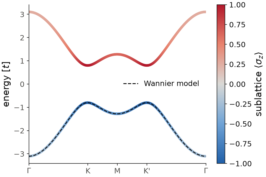
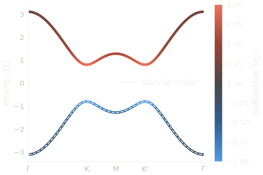
For the figure the bands of h are computed with operator="sublattice", so the color gives the sublattice polarization of each state. The valence band (blue) lives mostly on the sublattice with onsite energy \(-0.8\), and most strongly at K and K', where the gap is smallest, \(2\times0.8\). The band of the Wannier model (dashed) lies on top of the valence band along the whole path, from \(-3.10\) at \(\Gamma\) to \(-0.80\) at K. Its Wannier centre is at \((0.5,0)\), exactly on the site with onsite energy \(-0.8\), and its spread is \(\Omega=0.32\).

Code of this figure (documentation/figures/wannier_valence.py)

import numpy as np
import style
from pyqula import geometry
g = geometry.honeycomb_lattice()
h = g.get_hamiltonian(has_spin=False)
h.add_onsite([0.8,-0.8]) # sublattice potential opens a gap

# Wannierize just the lowest (valence) band: bands=[0,0] selects band
# index 0 at every k-point of a 12x12 Monkhorst-Pack wannierization mesh
hwan = h.get_wannier_hamiltonian(bands=[0,0],nk=12)

(k,e,sl) = h.get_bands(operator="sublattice",write=False) # colored by sublattice
(kw,ew) = hwan.get_bands(write=False)

def draw(ax, c):
    sc = ax.scatter(k, e, c=sl, s=10, cmap=c.diverging, vmin=-1, vmax=1)
    ax.plot(kw, ew, "--", color=c.ink, lw=1.4, label="Wannier model")
    style.colorbar(sc, ax, r"sublattice $\langle \sigma_z\rangle$")
    ticks = np.array([0, 1/3, 1/2, 2/3, 1])*max(k) # the path goes through K, M and K'
    ax.set_xticks(ticks, [r"$\Gamma$", "K", "M", "K'", r"$\Gamma$"])
    ax.set_xlim(0, max(k))
    ax.set_ylabel("energy [$t$]")
    ax.legend(loc="center right")

style.save(draw, "wannier_valence")

The mesh only fixes each hopping up to a translation by the supercell of nk cells. As in Wannier90, each hopping is put on the cell closest to the origin (the Wigner-Seitz cell of that supercell), so the Bloch Hamiltonian of the Wannier model is Hermitian at every k, also between mesh points.

See examples/wannier/get_wannier_hamiltonian/main.py for a runnable script, and jupyter-notebooks/functionalities/wannierization/01_maximally_localized_wannier.ipynb and 02_exact_reproduction.ipynb in the same folder for executed notebooks.

Symmetry-enforced Wannierization

The Wannier functions should respect the point-group symmetry of the lattice. With symmetries="auto", the point group is found from the geometry and the Hamiltonian, and the code first checks that the selected bands are a union of complete multiplets of this group at every k-point. If the selection cuts through a degeneracy protected by symmetry, the code raises a ValueError instead of returning a model with the wrong symmetry. A list of symmetrytk.pointgroup.SymmetryOperation can be given instead of "auto", to enforce only a subgroup.

The flat band of the kagome lattice is a good example. It is the lowest of the three bands, at \(E=-2\) in units of the hopping, and it touches the middle band at \(\Gamma\). So a selection with only the flat band is not a union of complete multiplets at \(\Gamma\). This touching is also the reason why the flat band alone has no exponentially localized Wannier functions:

from pyqula import geometry
from pyqula.symmetrytk import pointgroup

g = geometry.kagome_lattice()
h = g.get_hamiltonian(has_spin=False)

try:
    h.get_wannier_hamiltonian(bands=[0,0],nk=12,symmetries="auto") # the flat band alone
except ValueError as e:
    print("Flat band alone correctly rejected:",str(e).splitlines()[0])

# the full 3-band manifold has no such obstruction
hwan_sym = h.get_wannier_hamiltonian(bands=[0,2],nk=12,symmetries="auto")
print("Symmetries enforced:",[c.op.name for c in hwan_sym.wannier_symmetries])

The first call raises an error, and the message gives the symmetry and the k-point, \(\Gamma\), where the selection breaks a multiplet. The second call gives a model with three orbitals, whose Wannier functions transform into each other under the operations listed in wannier_symmetries.

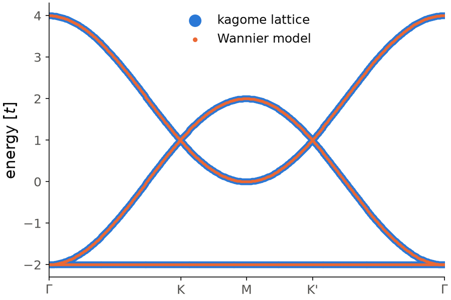
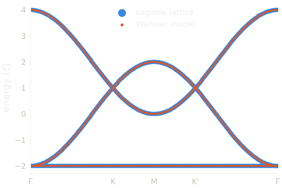
The three bands of the Wannier model (small orange dots) lie on the bands of the kagome lattice (blue): the flat band at \(E=-2\), the Dirac crossings at K and K' at \(E=1\), and the top of the band at \(E=4\) at \(\Gamma\). The largest difference between the two sets of energies along the path is \(4\times10^{-10}\). You also see the touching at \(\Gamma\) between the flat band and the middle band, which is the reason why the flat band alone is rejected.

Code of this figure (documentation/figures/wannier_kagome.py)

import numpy as np
import style
from pyqula import geometry
from pyqula.symmetrytk import pointgroup

g = geometry.kagome_lattice()
h = g.get_hamiltonian(has_spin=False)

try:
    h.get_wannier_hamiltonian(bands=[0,0],nk=12,symmetries="auto") # the flat band alone
except ValueError as e:
    print("Flat band alone correctly rejected:",str(e).splitlines()[0])

# the full 3-band manifold has no such obstruction
hwan_sym = h.get_wannier_hamiltonian(bands=[0,2],nk=12,symmetries="auto")
print("Symmetries enforced:",[c.op.name for c in hwan_sym.wannier_symmetries])

(k,e) = h.get_bands(write=False) # bands of the kagome lattice
(kw,ew) = hwan_sym.get_bands(write=False) # bands of the Wannier model

def draw(ax, c):
    ax.scatter(k, e, s=30, color=c.blue, label="kagome lattice")
    ax.scatter(kw, ew, s=3, color=c.orange, label="Wannier model")
    ticks = np.array([0, 1/3, 1/2, 2/3, 1])*max(k) # the path goes through K, M and K'
    ax.set_xticks(ticks, [r"$\Gamma$", "K", "M", "K'", r"$\Gamma$"])
    ax.set_xlim(0, max(k))
    ax.set_ylabel("energy [$t$]")
    ax.legend(loc="upper center", markerscale=2)

style.save(draw, "wannier_kagome")

See examples/wannier/symmetric_wannierization/main.py for a runnable script, and jupyter-notebooks/functionalities/wannierization/03_symmetry_enforced_wannierization.ipynb for the executed notebook.

Disentanglement

A selection of bands only works if these bands are separated from all the others by a gap in the whole Brillouin zone. Often they are not. The simplest case is graphene: its two \(p_z\) bands touch at K, so neither band alone is a smooth set of states. Disentanglement solves this. From a larger set of offered bands it extracts, at each k-point, the subspace of num_wann states that changes most smoothly with k, meaning that it minimizes the gauge-invariant part \(\Omega_I\) of the spread. This is the method of Souza, Marzari and Vanderbilt. It is switched on by giving a num_wann smaller than the number of selected bands; then bands=[a,b] only says which bands are offered.

import numpy as np
from pyqula import geometry
g = geometry.honeycomb_lattice()
h = g.get_hamiltonian(has_spin=False)

# one Wannier function out of both pz bands, with the deep part of the
# valence band frozen (kept exactly rather than optimized)
hwan = h.get_wannier_hamiltonian(bands=[0,1],num_wann=1,nk=12,
                                 dis_froz_max=-1.0,cutoff=0.0)

print("Wannier functions:",hwan.wannier_num_wann)
print("window used:",hwan.wannier_disentanglement_window)

f0,fw = h.get_hk_gen(),hwan.get_hk_gen()
k = [2./12.,1./12.,0.] # a wannierization-mesh k-point
e0 = np.sort(np.linalg.eigvalsh(f0(k))) ; ew = np.linalg.eigvalsh(fw(k))
print("frozen state reproduced to:",abs(ew[0]-e0[0]))

The model now reproduces exactly only the states inside the frozen window, below \(E=-1\) here, at every k-point of the mesh. Outside the frozen window it does not reproduce the offered bands: it follows a smoother subspace instead. So the last line prints a number at machine precision for the frozen valence state, while the conduction band is not in the model at all. This is the price of a smooth, localized orbital, not an error. With cutoff=0.0 all the real-space hoppings are kept; the default cutoff=1e-6 drops the small ones and changes the last digits.

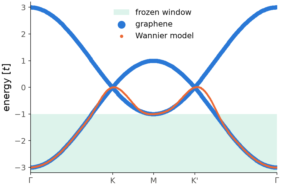
Below \(E=-1\) (shaded, the frozen window) the Wannier band (orange) is on top of the valence band of graphene (blue), from \(-3\) at \(\Gamma\) to \(-1\) at M. Above \(E=-1\) it leaves the valence band. Near K and K' it does not follow the kink of the Dirac cone; it goes smoothly through a maximum close to \(E=0\) instead. This smooth band is what makes the Wannier function localized. With these keywords the call also prints a warning, because the minimization of \(\Omega_I\) is not converged after the default 200 iterations; the frozen window is reproduced anyway.

Code of this figure (documentation/figures/wannier_disentangle.py)

import numpy as np
import style
from pyqula import geometry
g = geometry.honeycomb_lattice()
h = g.get_hamiltonian(has_spin=False)

# one Wannier function out of both pz bands, with the deep part of the
# valence band frozen (kept exactly rather than optimized)
hwan = h.get_wannier_hamiltonian(bands=[0,1],num_wann=1,nk=12,
                                 dis_froz_max=-1.0,cutoff=0.0)

print("Wannier functions:",hwan.wannier_num_wann)
print("window used:",hwan.wannier_disentanglement_window)

(k,e) = h.get_bands(write=False) # the two bands of graphene
(kw,ew) = hwan.get_bands(write=False) # the band of the Wannier model

def draw(ax, c):
    ax.axhspan(-3.2, -1.0, color=c.green, alpha=0.15, lw=0, label="frozen window")
    ax.scatter(k, e, s=30, color=c.blue, label="graphene")
    ax.scatter(kw, ew, s=4, color=c.orange, label="Wannier model")
    ticks = np.array([0, 1/3, 1/2, 2/3, 1])*max(k) # the path goes through K, M and K'
    ax.set_xticks(ticks, [r"$\Gamma$", "K", "M", "K'", r"$\Gamma$"])
    ax.set_xlim(0, max(k)) ; ax.set_ylim(-3.2, 3.2)
    ax.set_ylabel("energy [$t$]")
    ax.legend(loc="upper center", markerscale=2)

style.save(draw, "wannier_disentangle")

The keywords are:

• num_wann: number of Wannier functions; smaller than the number of selected bands switches on disentanglement.
• dis_froz_min, dis_froz_max: the frozen (inner) window; states inside it are reproduced exactly. Give both, or only dis_froz_max.
• dis_win_min, dis_win_max: the outer window; only the states inside it are offered at each k-point, so their number can change across the Brillouin zone.
• dis_num_iter: maximal number of iterations of the \(\Omega_I\) minimization (default 200); if it is not converged you get a warning, and the frozen window is reproduced anyway.

The returned Hamiltonian has the attributes wannier_num_wann and wannier_disentanglement_window (the four window values used, or None without disentanglement), together with the centres and spreads.

A window without a smaller num_wann, dis_froz_min without dis_froz_max, or a num_wann outside \(1\) to the number of bands raises an error, since the window would be ignored otherwise. Disentanglement does not work together with a Nambu (BdG) Hamiltonian, with symmetries=, or with auto_split_clusters=True; these combinations raise a NotImplementedError. Always give the window with the dis_* keywords and not through win_keywords=, since this last one is passed on without any check.

See jupyter-notebooks/functionalities/wannierization/04_dimensionality_and_bdg.ipynb for Wannierization in other dimensions and in the Nambu basis, and 05_band_disentanglement.ipynb in the same folder for disentanglement.