Single defects in infinite systems

We now see how to compute the effect of a single defect, an impurity or a vacancy, in an infinite crystal, with embedding.Embedding. A supercell calculation cannot do this exactly: the defect is repeated in every supercell, and it interacts with its own copies. The Green's function embedding keeps the infinite pristine crystal and changes only one cell.

Let \(H_0\) be the pristine periodic Hamiltonian, and \(G_0(E)\) its local Green's function on one unit cell,

\[G_0(E) = \frac{1}{N_k}\sum_k \left[E + i\delta - H_0(k)\right]^{-1}.\]

The rest of the infinite crystal acts on this cell as a self-energy \(\Sigma(E)\), defined by

\[G_0(E) = \left[E + i\delta - H_0^{\rm cell} - \Sigma(E)\right]^{-1},\]

where \(H_0^{\rm cell}\) is the pristine intracell Hamiltonian. The defect changes the Hamiltonian of this cell to \(V\), and the rest of the crystal is not changed, so the Green's function of the defective cell is the Dyson equation

\[G(E) = \left[E + i\delta - V - \Sigma(E)\right]^{-1}.\]

This is exact for a defect inside one cell, in a crystal that is infinite in all directions. The local density of states is \(\rho_n(E) = -\frac{1}{\pi}\,{\rm Im}\, G_{nn}(E)\), and around the defect it is what STM measures near a single adatom or vacancy.

In pyqula, h is the pristine Hamiltonian and m is a Hamiltonian with the defect; only its intracell matrix is used as \(V\). Here the defect is an onsite energy \(1.0\) on one site of a chain:

from pyqula import geometry
from pyqula import embedding
g = geometry.chain() # create the geometry
h = g.get_hamiltonian() # pristine, infinite Hamiltonian
hv = h.copy()
hv.add_onsite(lambda r: 1.0 if r[0]<0.01 else 0.0) # a single-site onsite defect
eb = embedding.Embedding(h,m=hv) # embed the defect in the infinite system
(x,y,d) = eb.get_ldos(energy=0.0,delta=1e-2,nsuper=200,nk=400) # LDOS around the defect

eb.get_ldos() returns the positions x, y of the sites in a window of nsuper unit cells around the defect, and the LDOS d on each of them, at the energy energy. The positions are half-integers, from \(-99.5\) to \(99.5\) here, and the defect is the site at \(x=0.5\). In a metal, as this chain, you see Friedel oscillations: the LDOS oscillates with wavevector \(2k_F\) around the defect. At \(E=0\) we have \(k_F=\pi/2\), so the LDOS alternates from one site to the next, between \(0.38\) and \(0.26\) next to the defect, with a converged k-mesh (see below). In one dimension the oscillation at a single energy does not decay with the distance. Here it decays slowly, to \(0.34\) and \(0.29\) at 90 sites from the defect, only because of the broadening \(\delta\), over a length of about \(v_F/(2\delta)=100\) sites. In a gapped system, a strong enough defect gives a bound state inside the gap, and its LDOS is localized around the defect.

The k-mesh has to resolve the broadening. With \(\delta=0.01\), nk=400 as in the snippet is not converged: next to the defect it gives \(0.49\) and \(0.29\) instead of \(0.38\) and \(0.26\), the values that nk=2000 and nk=8000 both give. So when you make delta smaller, make nk larger, and compare two values of nk. The call also writes LDOS.OUT; pass write=False to avoid it.

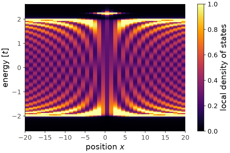
For the figure we compute the same LDOS at 105 energies, on the 40 sites around the defect, and with the converged nk=2000 instead of 400. The defect is at \(x=0.5\). Inside the band, between \(-2\) and \(2\), you see the Friedel oscillations as a checkerboard. At \(E=0\) the Fermi momentum is \(k_F=\pi/2\), so the period is two sites, \(2k_F=\pi\), and at other energies the period follows \(k_F\). Over these 40 sites the amplitude decays only a little, as we saw above. Above the band, at \(E=2.25\), there is a bright spot on the defect: the repulsive onsite energy \(V=1\) pulls one state out of the band, a bound state at \(\sqrt{4t^2+V^2}=2.24\).

Code of this figure (documentation/figures/embedding_ldos.py)

import numpy as np
import style
from pyqula import geometry
from pyqula import embedding
g = geometry.chain() # create the geometry
h = g.get_hamiltonian() # pristine, infinite Hamiltonian
hv = h.copy()
hv.add_onsite(lambda r: 1.0 if r[0]<0.01 else 0.0) # a single-site onsite defect
eb = embedding.Embedding(h,m=hv) # embed the defect in the infinite system
(x,y,d) = eb.get_ldos(energy=0.0,delta=1e-2,nsuper=200,nk=400) # LDOS around the defect

# the same LDOS at many energies, on 40 sites and with a finer k-mesh
es = np.linspace(-2.6,2.6,105)
ldos = np.array([eb.get_ldos(energy=e,delta=1e-2,nsuper=40,nk=2000)[2] for e in es])
x40 = eb.get_ldos(energy=0.,delta=1e-2,nsuper=40,nk=2000)[0] # positions of the 40 sites

def draw(ax, c):
    m = ax.pcolormesh(x40, es, ldos, cmap=c.cmap, vmin=0, vmax=1, shading="nearest")
    style.colorbar(m, ax, "local density of states")
    ax.set_xlabel("position $x$")
    ax.set_ylabel("energy [$t$]")

style.save(draw, "embedding_ldos")

The other methods of the embedding object:

• eb.get_dos(): the total DOS of the window around the defect.
• eb.multildos(): the LDOS at many energies, written to the folder MULTILDOS/.
• eb.get_gf(): the Green's function \(G(E)\) of the defective cell.
• eb.get_didv(): the differential conductance of an STM tip on the defect.

The momentum-space picture of the same defect is Quasiparticle interference. See examples/embedding/single_impurity_1D/main.py and examples/embedding/honeycomb_vacancy/main.py for runnable scripts, the other scripts in examples/embedding/ for vacancies, boundaries and Yu-Shiba-Rusinov states, and jupyter-notebooks/functionalities/spectral_functions/04_single_impurities_infinite.ipynb for an executed notebook.