Altermagnets

An altermagnet is a collinear magnet with zero net magnetization, but with spin-up and spin-down bands that are different. The two spin channels are related by a rotation or a mirror of the lattice, not by a translation or by inversion, so the spin splitting changes sign in reciprocal space, with d-wave, g-wave or i-wave symmetry. In this page we see how to measure how large the spin splitting is, and how to find its symmetry from the nonlinear spin current.

Spin splitting of an altermagnet

When spin is a good quantum number, the Bloch Hamiltonian has one block per spin, and we can diagonalize each block alone. This gives energies \(E^\uparrow_n(\mathbf k)\) and \(E^\downarrow_n(\mathbf k)\), sorted by band index \(n\). For each \(\mathbf k\) and \(n\) we define the spin splitting and its mean energy,

\[ \Delta_n(\mathbf k) = E^\uparrow_n(\mathbf k) - E^\downarrow_n(\mathbf k), \qquad \bar E_n(\mathbf k) = \frac{E^\uparrow_n(\mathbf k) + E^\downarrow_n(\mathbf k)}{2} . \]

The splitting is what spin-resolved ARPES sees as the energy difference of the two spin bands. pyqula gives two functions of energy built from the pairs \((\bar E_n(\mathbf k), \Delta_n(\mathbf k))\) on a k-mesh of the whole Brillouin zone:

• h.get_spin_splitting_vs_energy(): the largest \(|\Delta_n(\mathbf k)|\) in each energy bin. Its maximum is the largest spin splitting anywhere in the Brillouin zone.
• h.get_spin_splitting_density(): each pair broadened with a width delta, giving a smooth weighted density, the typical splitting at each energy.

To quote one number for a material, use the first one. The maximum along a single cut in reciprocal space (a circle, say) depends on where you look; the maximum over the full mesh does not.

import numpy as np
from pyqula import specialhamiltonian

h = specialhamiltonian.square_altermagnet(am=1.)

# largest spin splitting in each energy bin, over the whole BZ
(es, ds) = h.get_spin_splitting_vs_energy(nk=800, nbins=400)
print("largest spin splitting anywhere in the BZ:", ds.max())

# the smooth counterpart, on the same axes
(xs, ys) = h.get_spin_splitting_density(nk=100, delta=1e-1, energies=es)

Both return (energies, values) with the same shape, so they can be plotted together. An energy bin without states gives 0.0.

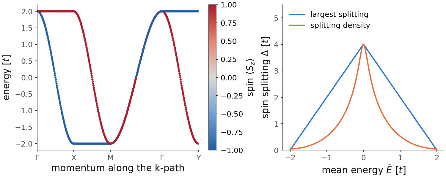
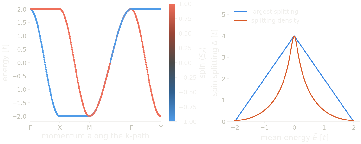
The left panel shows the bands of this model along the path \(\Gamma\)-X-M-\(\Gamma\)-Y, colored by the spin of each state with h.get_bands(operator="sz"). With am=1 the spin-up electrons hop only along \(y\) and the spin-down electrons only along \(x\), so \(E^\uparrow=2\cos k_y\) and \(E^\downarrow=2\cos k_x\). Along \(\Gamma\)-X the spin-up band (red) is flat at \(2\) and the spin-down band (blue) goes down to \(-2\). Along \(\Gamma\)-Y it is the opposite, and along M-\(\Gamma\) the two bands are the same. This sign change of the splitting between the two directions is the d-wave symmetry. The right panel is the output of the snippet. The largest splitting is \(4.0\), at mean energy \(0\), which is the X point, where \(E^\uparrow=2\) and \(E^\downarrow=-2\). The largest splitting per bin (blue) is the triangle \(\Delta_{\rm max}=4-2|\bar E|\). At a fixed mean energy the splitting is largest when one spin sits at the top of its band, at \(2\), so \(E^\uparrow-E^\downarrow=2-(2\bar E-2)=4-2\bar E\) for \(\bar E>0\). This curve needs a fine mesh, because each of the 400 bins must hold a k-point close to where its maximum is reached. With nk=100 many bins fall far below the triangle, and some are empty and give zero. With nk=800 every bin is within \(0.005\) of the triangle, and nk=1600 changes nothing visible. This takes about a minute. The density (orange) is smooth, with the same maximum, and it is already converged at nk=100.

Code of this figure (documentation/figures/altermagnets_splitting.py)

import numpy as np
import style
from pyqula import specialhamiltonian

h = specialhamiltonian.square_altermagnet(am=1.)

# largest spin splitting in each energy bin, over the whole BZ
(es, ds) = h.get_spin_splitting_vs_energy(nk=800, nbins=400)
print("largest spin splitting anywhere in the BZ:", ds.max())

# the smooth counterpart, on the same axes
(xs, ys) = h.get_spin_splitting_density(nk=100, delta=1e-1, energies=es)

nodes = np.array([[0,0,0],[.5,0,0],[.5,.5,0],[0,0,0],[0,.5,0]]) # Gamma X M Gamma Y
n = [int(200*np.linalg.norm(b-a)) for (a,b) in zip(nodes,nodes[1:])] # points per segment
kpath = np.concatenate([np.linspace(a,b,m,endpoint=False) for (a,b,m) in zip(nodes,nodes[1:],n)])
(k,e,sz) = h.get_bands(operator="sz", kpath=kpath) # bands, and the spin of each state
ticks = np.cumsum([0]+n) # index of each high-symmetry point

def draw(axs, c):
    ax = axs[0]
    sc = ax.scatter(k, e, c=sz, s=6, cmap=c.diverging, vmin=-1, vmax=1)
    style.colorbar(sc, ax, r"spin $\langle S_z\rangle$")
    ax.set_xticks(ticks, [r"$\Gamma$", "X", "M", r"$\Gamma$", "Y"])
    ax.set_xlim(0, ticks[-1])
    ax.set_xlabel("momentum along the k-path")
    ax.set_ylabel("energy [$t$]")
    ax = axs[1]
    ax.plot(es, ds, color=c.blue, label="largest splitting")
    ax.plot(xs, ys, color=c.orange, label="splitting density")
    ax.set_xlabel("mean energy $\\bar E$ [$t$]")
    ax.set_ylabel("spin splitting $\\Delta$ [$t$]")
    ax.set_ylim(0, 5.5)
    ax.legend(loc="upper left")

style.save(draw, "altermagnets_splitting", npanels=2)

The bands are paired by their index \(n\), and you may ask if the \(n\)-th up band and the \(n\)-th down band are really partners. In an altermagnet this is safe. The two spin channels are related by a point-group operation \(R\), so \(E^\uparrow_n(\mathbf k) = E^\downarrow_n(R\mathbf k)\) exactly, and \(\Delta_n(\mathbf k) = E^\downarrow_n(R\mathbf k) - E^\downarrow_n(\mathbf k)\) compares the same band at two momenta. This holds even when the splitting is larger than the distance between bands. For the square altermagnet \(R\) is the mirror \(k_1 \leftrightarrow k_2\).

There is one case where the pairing gives a wrong number: a unit cell larger than the magnetic unit cell. In a supercell, the bands at one \(\mathbf k\) come from several k-points of the primitive cell, and pairing them by index mixes them. The maximum then comes out too small. So use the true magnetic unit cell. If the magnetic order repeats with a shorter period than the cell you used, the result is only a lower bound.

Both functions need spin to be a good quantum number. h.get_spin_splitting_vs_energy() raises an error if the Bloch Hamiltonian mixes the two spins, as with Rashba coupling, other spin-orbit coupling, or non-collinear magnetic order. In these cases \(\Delta_n\) is not defined.

See examples/2d/spin_splitting_vs_energy/main.py for a runnable script that plots both curves and shows the problem of a too large cell, examples/2d/altermagnetism_density/main.py for the density alone, and jupyter-notebooks/functionalities/single_particle_hamiltonians/11_altermagnet_spin_splitting.ipynb for an executed notebook.

Nonlinear spin current as a measurement of altermagnetic order

The spin splitting tells how large the altermagnetic order is. We now ask which kind it is, d-wave, g-wave or i-wave. The answer can be found with a purely electrical measurement, without spin-orbit coupling: the lowest order in the electric field at which a spin current appears. This is computed with h.get_nonlinear_drude_orders().

The spin splitting of an X-wave magnet is a lattice harmonic of order \(l+1\) in \(\mathbf k\): \(k_xk_y\) for d-wave, \(k_xk_y(k_x^2-k_y^2)\) for g-wave, \(k_xk_y(3k_x^2-k_y^2)(k_x^2-3k_y^2)\) for i-wave. In the semiclassical Boltzmann theory, with relaxation time \(\tau\) and frequency \(\omega\), the current of spin \(s\) at order \(l=l_1+l_2\) in the field, \(j_b = \sigma_s^{x^{l_1}y^{l_2};b} E_x^{l_1}E_y^{l_2}\), has the conductivity

\[ \sigma_s^{x^{l_1} y^{l_2};b} = \frac{(-e/\hbar)^{l+1}}{(i\omega + 1/\tau)^{l}} \int \frac{d^D k}{(2\pi)^D}\, f_s^{(0)}(\mathbf k)\, \frac{\partial^{l+1} \epsilon_s(\mathbf k)}{\partial k_x^{l_1}\, \partial k_y^{l_2}\, \partial k_b} , \]

where \(\epsilon_s(\mathbf k)\) is the band of spin \(s\), \(f_s^{(0)}\) its Fermi occupation, and \(b\) the direction of the current. The spin and charge conductivities are

\[ \sigma_{\rm spin} = \frac{\sigma_\uparrow - \sigma_\downarrow}{2}, \qquad \sigma_{\rm charge} = \sigma_\uparrow + \sigma_\downarrow . \]

A harmonic of order \(l+1\) has a constant \((l+1)\)-th derivative, and all lower derivatives vanish after the integral over the zone. So the spin current appears for the first time at one order \(l\), and is exactly zero below it:

wave	d	f	g	i
lowest order l	1	2	3	5

The p-wave magnet, with splitting \(\propto k_x\), would be at \(l=0\), but it has no spin current at any order. First, the order \(l=0\) is zero for every band: the integrand \(f\,\partial\epsilon/\partial k_b\) is a total derivative, so there is no current in equilibrium. Second, on the lattice the p-wave splitting \(J\sin k_x\) and the hopping \(2t\cos k_x\) combine into a single cosine of amplitude \(\sqrt{4t^2+J^2}\), so the two spin bands are the same band shifted along \(k_x\) in opposite directions, and an integral over the zone does not see a shift. On a finite k-mesh these two zeros are small numbers instead of exact zeros: at nk=48 the p-wave magnet gives \(3\times10^{-4}\) at the even orders, and this goes down exponentially with nk, to \(10^{-11}\) at nk=384. The zeros below the threshold of the d-, f-, g- and i-wave magnets come from symmetry and are exact on any mesh. So a number that becomes smaller when you increase nk is a zero, not the threshold.

So the lowest order with a nonzero spin current gives the wave index. This is the proposal of Ezawa, Phys. Rev. B 111, 125420 (arXiv:2411.16036). For an i-wave altermagnet:

from pyqula import specialhamiltonian

h = specialhamiltonian.iwave_altermagnet(J=0.3)   # or dwave_/fwave_/gwave_

# largest |sigma_spin| over every component of each order l
orders = h.get_nonlinear_drude_orders(lmax=6, nk=48, T=0.02, mu=-5.5)
# -> zero to machine precision for l = 0..4, nonzero at l = 5

# one component, and every component of a given order
s = h.get_nonlinear_drude_conductivity(field="yyyyy", current="x", mu=-5.5)
c = h.get_nonlinear_drude_components(5, nk=48, mu=-5.5)   # {"x^l1 y^l2;b": value}

h.get_nonlinear_drude_orders() returns, for each order l up to lmax, the largest \(|\sigma_{\rm spin}|\) over all the components of that order. Here it is zero (to machine precision) for l from 0 to 4 and nonzero at l = 5, the fingerprint of i-wave order. The keywords are:

• field: one character per power of the electric field, so "yyyyy" is the fifth-order response to \(E_y\).
• current: the direction \(b\) of the current.
• channel: "spin" (default), "charge", "up" or "dn".
• mu, T: the chemical potential and the temperature of \(f^{(0)}\).
• nk: the k-mesh, per direction.

Units are \(e=\hbar=1\), and the integral is normalized per unit area (or volume), \(\int d^Dk/(2\pi)^D\).

The models are specialhamiltonian.xwave_magnet(wave=...), with the names pwave_magnet, dwave_altermagnet, fwave_magnet, gwave_altermagnet and iwave_altermagnet. These are Ezawa's models, each on the lattice its symmetry needs: square for p, d and g, triangular for f and i.

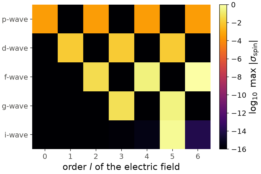
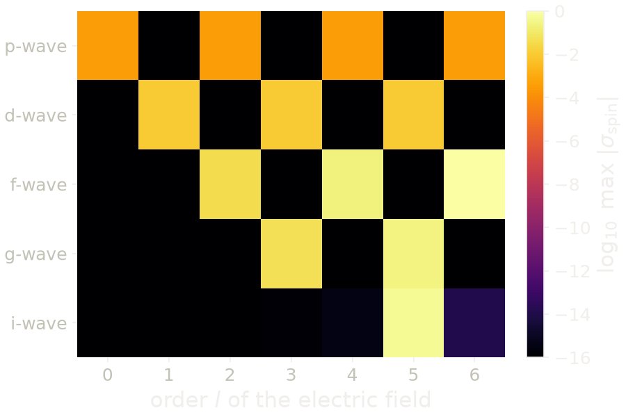
Each row is one model of specialhamiltonian.xwave_magnet(), with \(J=0.3\) and the chemical potential \(0.5\) above the bottom of its band, as \(\mu=-5.5\) in the snippet for the i-wave one. The color is \(\log_{10}\) of the output of h.get_nonlinear_drude_orders(), and the zeros are drawn at \(10^{-16}\). In each row, the first bright cell is the threshold of the table: \(l=1\) for d-wave (\(0.011\)), \(l=2\) for f-wave (\(0.041\)), \(l=3\) for g-wave (\(0.053\)) and \(l=5\) for i-wave (\(0.56\)). Every cell below it is black, an exact zero. The d-, f- and g-wave rows also respond at higher orders, the higher harmonics. The p-wave row is the mesh error discussed above: \(3\times10^{-4}\) at the even orders at nk=48, and it goes down when you increase nk.

Code of this figure (documentation/figures/altermagnets_orders.py)

import numpy as np
import style
from pyqula import specialhamiltonian

h = specialhamiltonian.iwave_altermagnet(J=0.3)   # or dwave_/fwave_/gwave_

# largest |sigma_spin| over every component of each order l
orders = h.get_nonlinear_drude_orders(lmax=6, nk=48, T=0.02, mu=-5.5)
# -> zero to machine precision for l = 0..4, nonzero at l = 5

# one component, and every component of a given order
s = h.get_nonlinear_drude_conductivity(field="yyyyy", current="x", mu=-5.5)
c = h.get_nonlinear_drude_components(5, nk=48, mu=-5.5)   # {"x^l1 y^l2;b": value}

# the same for every model, with mu 0.5 above the bottom of its band
waves = {"p":-3.5, "d":-3.5, "f":-5.5, "g":-3.5, "i":-5.5} # wave: mu
table = [specialhamiltonian.xwave_magnet(wave=w,J=0.3,t=-1.).get_nonlinear_drude_orders(
         lmax=6, nk=48, T=0.02, mu=mu) for (w,mu) in waves.items()]
logs = np.log10(np.maximum(np.array(table), 1e-16)) # zeros drawn at 1e-16

def draw(ax, cl):
    m = ax.imshow(logs, cmap=cl.cmap, vmin=-16, vmax=0, aspect="auto")
    style.colorbar(m, ax, r"$\log_{10}$ max $|\sigma_{\rm spin}|$")
    ax.set_xticks(range(7))
    ax.set_yticks(range(len(waves)), [w+"-wave" for w in waves])
    ax.set_xlabel("order $l$ of the electric field")
    ax.spines[:].set_visible(False)

style.save(draw, "altermagnets_orders")

Some things to keep in mind before using the result:

• The orders above the threshold are not zero. A lattice harmonic also contains higher harmonics, so a d-wave altermagnet responds at l = 1, and also at l = 3 and l = 5. The information is in the absence of all the orders below the threshold.
• An insulator gives zero at every order. With the chemical potential in the gap, every band is full or empty, and the integral vanishes, also at fifth order. So "nothing below fifth order" says i-wave only if the fifth order is nonzero, which needs a metal.
• A spin-degenerate state has no spin current. A compensated Néel state on a bipartite lattice has \(PT\) symmetry and its two spin channels are exactly degenerate: it is an antiferromagnet, not an altermagnet. In this case the result is numerical noise that does not look small, so a warning is raised when the spin splitting is below \(10^{-10}\) of the bandwidth.

Real hoppings also give a selection rule, useful when building a model. With real hoppings and no spin-orbit coupling, \(\epsilon_s(\mathbf k)=\epsilon_s(-\mathbf k)\), so the splitting is even under a rotation by \(180^\circ\) and all odd harmonics vanish. A \(C_3\) axis also removes every harmonic whose order is not a multiple of three. Only the orders \(6, 12, \dots\) survive, which is \(l=5, 11, \dots\). So a real, spin-orbit-free cell with \(C_3\) symmetry is always i-wave, and no pattern of vacancies or supercell can make it f-wave. The models agree with this: p-wave and f-wave need complex hoppings, while d-, g- and i-wave are real.

Spin must be a good quantum number, because the formula treats each spin channel alone. A Hamiltonian with spin-orbit coupling is rejected: with Rashba or Kane-Mele terms the nonlinear response has extra contributions from the quantum metric and the Berry curvature dipole (arXiv:2409.09241), which are not in this formula.

Unit cells with many orbitals (superlattices, antidot lattices, multilayers) are supported, and they are the interesting case. The derivatives of the bands are computed analytically, also at the degeneracies that a \(C_3\) or \(C_6\) axis creates at high-symmetry points, so an order forbidden by symmetry comes out as an exact zero.

See examples/2d/xwave_nonlinear_spin_current/main.py for a runnable script that prints the whole table, and jupyter-notebooks/functionalities/single_particle_hamiltonians/12_nonlinear_spin_conductivity.ipynb for an executed notebook.