Spectral functions and Fermi surfaces

In this page we compute the spectral function resolved in momentum and energy: along a k-path, on a constant-energy cut of the Brillouin zone (the Fermi surface), and at the surface of a semi-infinite crystal. These are the quantities that ARPES measures.

Momentum-resolved spectral function

The band structure gives the energies as sharp lines. The momentum-resolved spectral function gives the same information as a heatmap, where each band has a finite width and can be weighted by an operator \(O\),

\[ A_O(k,\omega) = -\frac{1}{\pi}\,\textrm{Im}\,\textrm{Tr}\left[O\,G(k,\omega+i\delta)\right] = \sum_\alpha \langle \Psi_{k,\alpha}|O|\Psi_{k,\alpha}\rangle\, \delta(\omega-\epsilon_{k,\alpha}) , \]

where \(G(k,z)=(z-H_k)^{-1}\) is the Green's function, \(\epsilon_{k,\alpha}\) and \(\Psi_{k,\alpha}\) are the eigenenergies and eigenstates at momentum \(k\), and the delta function is a Lorentzian of width \(\delta\). Without an operator, \(O\) is the identity and \(A(k,\omega)\) is the total spectral weight. This is the band structure as ARPES sees it. The operator is useful to select a part of the states. For example, in a superconductor the projector on the electron sector gives the electron spectral function, without the hole copy of the bands. We compute it with h.get_kdos_bands():

from pyqula import geometry
g = geometry.triangular_lattice() # get the geometry
h = g.get_hamiltonian()  # get the Hamiltonian
h.get_kdos_bands()

h.get_kdos_bands() returns three arrays: the position along the k-path, the energy, and \(A(k,\omega)\) at each pair. By default the energies go from \(-3\) to \(3\). The same three columns are written to KDOS_BANDS.OUT. The broadening delta is the width of each line in the heatmap.

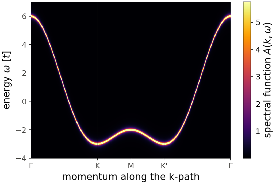
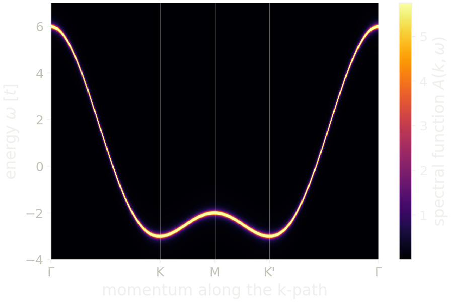
For the figure we take energies=np.linspace(-4,7,1101), because the default window from \(-3\) to \(3\) cuts the band. We also take nk=600 points on the k-path and delta=0.05. The energy step, \(0.01\), and the change of the band energy between two k-points must both be smaller than delta, otherwise the line breaks into separate dots. You see the single band of the triangular lattice, from \(-3t\) at K and K' to \(6t\) at \(\Gamma\), with a local maximum at \(-2t\) at M, the saddle point. The width of the line is the broadening.

Code of this figure (documentation/figures/spectral_kdos.py)

import numpy as np
import style
from pyqula import geometry

g = geometry.triangular_lattice() # get the geometry
h = g.get_hamiltonian()  # get the Hamiltonian
(k,e,d) = h.get_kdos_bands(energies=np.linspace(-4,7,1101),nk=600,delta=0.05) # the whole band, on a dense path

nk, ne = len(np.unique(k)), len(np.unique(e)) # k is the outer index
(k,e,d) = [a.reshape(nk,ne) for a in (k,e,d)]

def draw(ax, c):
    im = ax.pcolormesh(k, e, d, cmap=c.cmap, shading="auto", vmax=np.percentile(d,99))
    style.colorbar(im, ax, r"spectral function $A(k,\omega)$")
    style.kpath(ax, k, [r"$\Gamma$", "K", "M", "K'", r"$\Gamma$"], at=[0,1/3,1/2,2/3,1])
    ax.set_xlabel("momentum along the k-path")
    ax.set_ylabel(r"energy $\omega$ [$t$]")

style.save(draw, "spectral_kdos")

The keywords are

• energies: the energies \(\omega\).
• delta: the broadening \(\delta\).
• operator: the operator \(O\).
• kpath, nk: the k-path and the number of k-points, as in h.get_bands().
• mode: "ED" (default, diagonalization), "green" (Green's function) or "KPM" (Chebyshev expansion, for large systems).

The three modes give the same quantity with the same normalization, so a system that is too large to diagonalize can go from mode="ED" to mode="KPM" without changing the scale. Only the line shape changes: the Chebyshev expansion broadens each band with its kernel, not with a Lorentzian of width delta.

See examples/1d/kdos_armchair/main.py for a runnable script on a wide ribbon with mode="KPM", and jupyter-notebooks/functionalities/single_particle_hamiltonians/05_momentum_resolved_spectral_functions.ipynb and jupyter-notebooks/functionalities/spectral_functions/06_operator_momentum_resolved.ipynb for executed notebooks.

Fermi surface

The Fermi surface is the set of momenta where a band crosses the Fermi energy. It is what a metal looks like in reciprocal space, and it controls the low-temperature transport and the nesting instabilities. For a 2D Hamiltonian, h.get_fermi_surface() computes the spectral weight \(A(\mathbf k,\omega=E)\) on a \((k_x,k_y)\) mesh, at one energy \(E\) (by default the Fermi energy, e=0.0). It is a constant-energy cut of the spectral function, as measured by ARPES:

from pyqula import geometry
g = geometry.triangular_lattice() # get the geometry
h = g.get_hamiltonian() # get the Hamiltonian
(kx,ky,fs) = h.get_fermi_surface(e=0.0,nk=50,delta=1e-1)

It returns the two coordinates of each point of the mesh and the spectral weight at that point. A scatter plot colored by the weight shows the Fermi surface. The broadening delta sets the thickness of the contour. If delta is smaller than the energy spacing of the k-mesh, you see the mesh and not the contour.

The keywords are

• e: the energy of the cut.
• nk: number of k-points per direction.
• delta: the broadening.
• operator: weight each state with an operator, which gives for example a spin or valley texture of the Fermi surface.

With an operator, each point is weighted with the expectation value of the operator. This is how we see the spin texture of a material with spin-orbit coupling. The NbSe2 Hamiltonian below is a multi-orbital model with spin-orbit coupling, and the weight \(\langle s_z\rangle\) tells apart the two spin channels on each pocket:

from pyqula.specialhamiltonian import NbSe2
h = NbSe2(soc=0.9) # multi-orbital spin-orbit-coupled Hamiltonian
(kx,ky,fs) = h.get_fermi_surface(e=0.,nk=100,delta=3e-1,operator="sz")

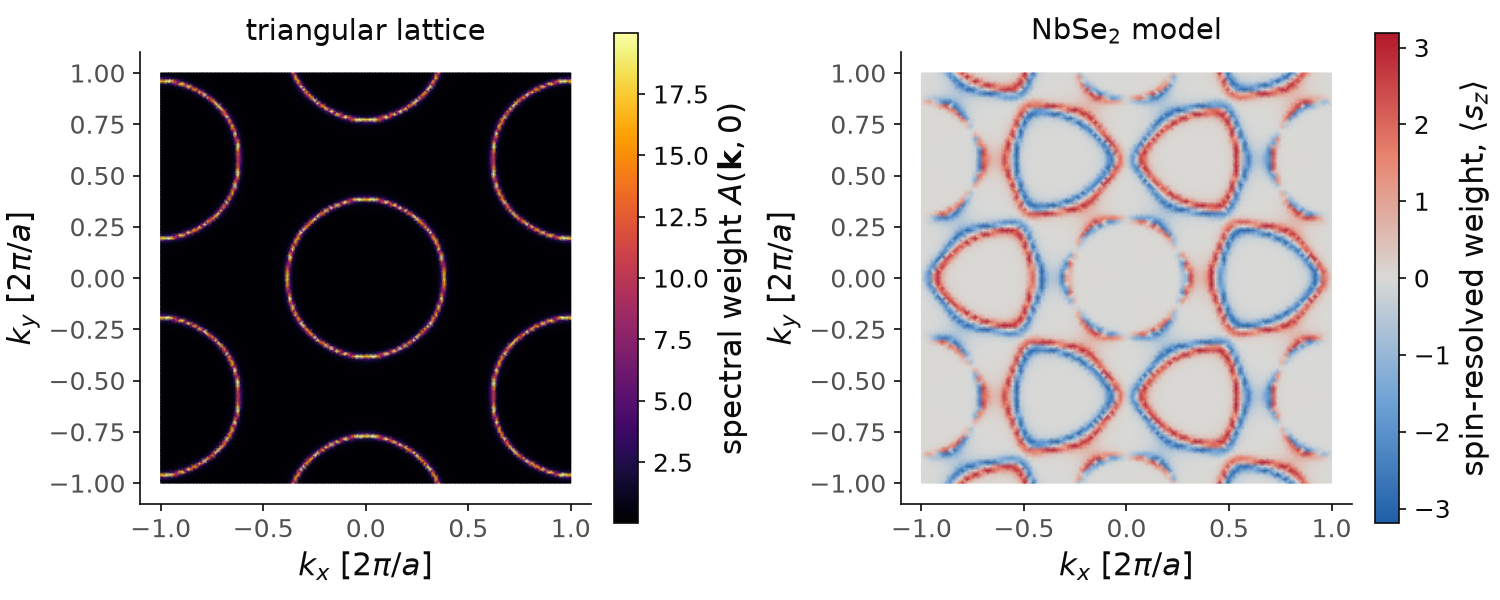
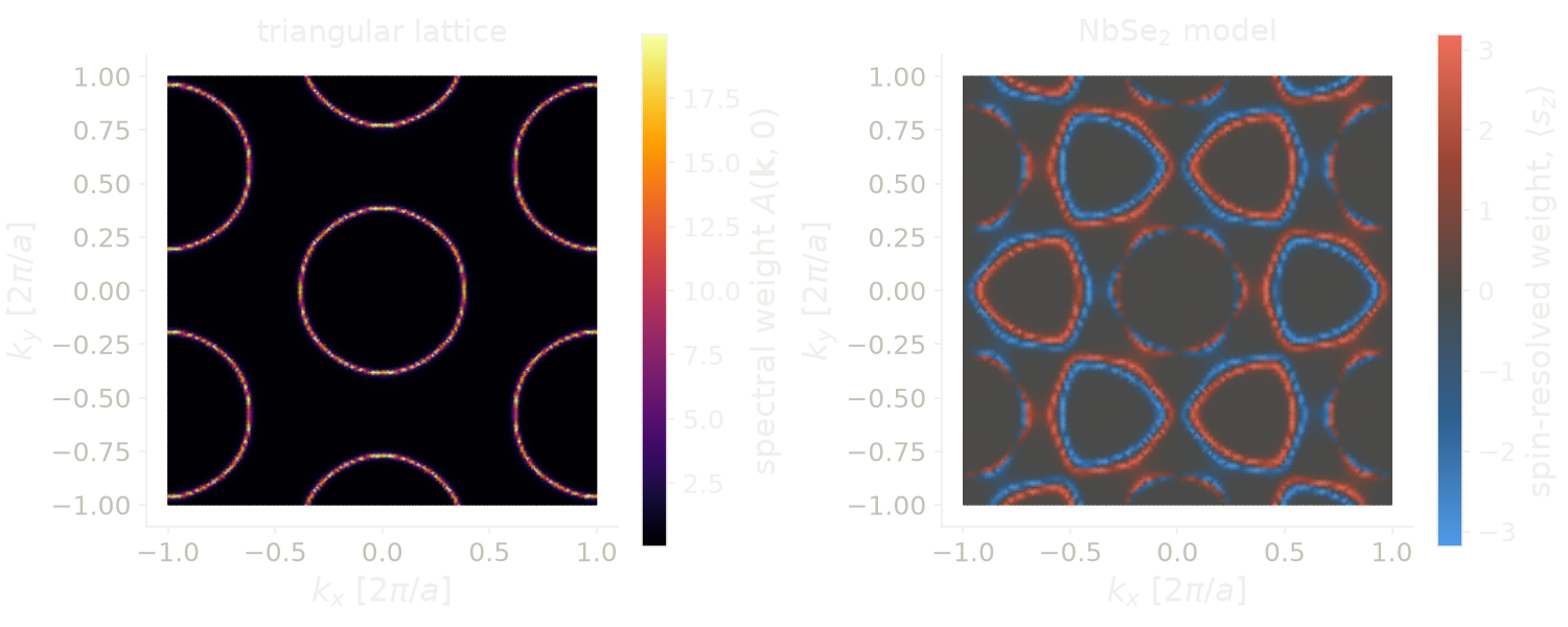
The momenta are Cartesian, in units of \(2\pi/a\). On the left, the Fermi surface of the triangular lattice at zero energy is a circle of radius \(0.38\) around \(\Gamma\), repeated around the neighboring reciprocal lattice points. For the figure we take nk=150 instead of nk=50: with nk=50 and delta=1e-1 the contour breaks into dots, which is the k-mesh and not the physics. On the right, the NbSe2 model has a pocket around \(\Gamma\) and pockets around K and K', at \(k_x=\pm 0.67\). Each pocket at K and K' is split in two by the spin-orbit coupling, with opposite \(\langle s_z\rangle\), and the order of the two colors is reversed between K and K'. This is the Ising spin-orbit coupling of NbSe2. The pocket around \(\Gamma\) has a much weaker spin texture.

Code of this figure (documentation/figures/spectral_fermi.py)

import numpy as np
import style
from pyqula import geometry
from pyqula.specialhamiltonian import NbSe2

g = geometry.triangular_lattice() # get the geometry
h = g.get_hamiltonian() # get the Hamiltonian
(kx,ky,fs) = h.get_fermi_surface(e=0.0,nk=150,delta=1e-1)

h = NbSe2(soc=0.9) # multi-orbital spin-orbit-coupled Hamiltonian
(kx2,ky2,fs2) = h.get_fermi_surface(e=0.,nk=100,delta=3e-1,operator="sz")

def draw(ax, c):
    im = ax[0].tripcolor(kx, ky, fs, cmap=c.cmap, shading="gouraud")
    style.colorbar(im, ax[0], r"spectral weight $A(\mathbf{k},0)$")
    ax[0].set_title("triangular lattice")
    m = np.abs(fs2).max()
    im = ax[1].tripcolor(kx2, ky2, fs2, cmap=c.diverging, vmin=-m, vmax=m, shading="gouraud")
    style.colorbar(im, ax[1], r"spin-resolved weight, $\langle s_z\rangle$")
    ax[1].set_title(r"NbSe$_2$ model")
    for a in ax:
        a.set_aspect("equal")
        a.set_xlabel(r"$k_x$ [$2\pi/a$]")
        a.set_ylabel(r"$k_y$ [$2\pi/a$]")

style.save(draw, "spectral_fermi", npanels=2)

h.get_multi_fermi_surface() computes the same map at many energies, and writes one file per energy to the folder MULTIFERMISURFACE/. This shows how the constant-energy contours change away from the Fermi energy:

import numpy as np
h.get_multi_fermi_surface(energies=np.linspace(-4,4,100),delta=1e-1)

Unfolded Fermi surface of a supercell

A defect or a charge order needs a supercell, and the Fermi surface of a supercell is folded into its small Brillouin zone. With operator="unfold", the spectral weight is projected back onto the Brillouin zone of the primitive cell, as ARPES sees it (see Band unfolding for the formula). The supercell must be built with store_primal=True, and nsuper stretches the mesh over the primitive Brillouin zone:

import numpy as np
from pyqula import geometry
g0 = geometry.triangular_lattice()
n = 3 # size of the supercell
g = g0.get_supercell(n,store_primal=True)
h = g.get_hamiltonian()
h.add_onsite(lambda r: 100.0 if np.linalg.norm(r-g.r[0])<1e-1 else 0.0) # a point defect

out = h.get_multi_fermi_surface(nk=50,energies=np.linspace(-4,4,100),delta=0.1,
        nsuper=n,operator="unfold")

nsuper=n works for a supercell with the same shape as the primitive cell. For a supercell with another shape, the mesh comes out sheared. For any supercell, use primal_mesh=True instead. The mesh is then drawn in the Brillouin zone of the primitive cell, and each point is computed at the equivalent momentum of the supercell:

import numpy as np
from pyqula import geometry
g0 = geometry.triangular_lattice() # primitive geometry
g = g0.get_supercell(np.sqrt(3),store_primal=True) # sqrt(3) x sqrt(3) supercell
h = g.get_hamiltonian() # Hamiltonian of the supercell
h.add_onsite(lambda r: 0.6 if np.linalg.norm(r-g.r[0])<1e-1 else 0.0) # charge order
(kx,ky,fs) = h.get_fermi_surface(e=0.0,nk=50,delta=0.1,operator="unfold",
        primal_mesh=True) # unfolded Fermi surface, on the primitive mesh

The result is on the same mesh and in the same coordinates as the Fermi surface of the primitive cell, so the two can be compared point by point. For a supercell without any modulation, the two maps are the same, up to a factor equal to the number of primitive cells in the supercell. Note that a supercell with a non-integer size, as \(\sqrt 3\) here, is rotated so that its first lattice vector is along \(x\), and its Fermi surface is drawn in this rotated frame.

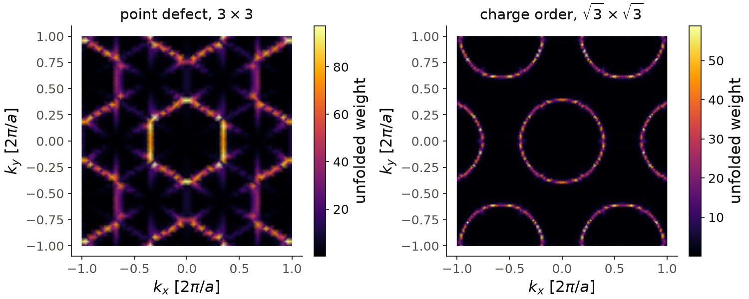
Both maps are at zero energy, in units of \(2\pi/a\) of the primitive cell. On the left, the frame of h.get_multi_fermi_surface() closest to zero energy, \(\omega=-0.04t\), with the mesh divided by n to have the same units. The point defect is strong, one site in nine, and the circle of the clean lattice becomes a hexagon of about the same size, with weak shadow lines of the folded copies around it. On the right, the charge order of \(0.6\) leaves the circle of radius \(0.38\) almost unchanged at this energy. The neighboring circles are around \((\pm 1.15,0)\) and \((\pm 0.58,\pm 1)\), the reciprocal lattice of the rotated frame. For the figure we take nk=100 instead of nk=50, so that the circle is a smooth line. The largest weight is \(58\), three times the one of the primitive cell, as expected for three primitive cells in the supercell.

Code of this figure (documentation/figures/spectral_unfoldfs.py)

import numpy as np
import style
from pyqula import geometry

# point defect in a 3 x 3 supercell
g0 = geometry.triangular_lattice()
n = 3 # size of the supercell
g = g0.get_supercell(n,store_primal=True)
h = g.get_hamiltonian()
h.add_onsite(lambda r: 100.0 if np.linalg.norm(r-g.r[0])<1e-1 else 0.0) # a point defect

out = h.get_multi_fermi_surface(nk=50,energies=np.linspace(-4,4,100),delta=0.1,
        nsuper=n,operator="unfold")

# charge order in a sqrt(3) x sqrt(3) supercell
g0 = geometry.triangular_lattice() # primitive geometry
g = g0.get_supercell(np.sqrt(3),store_primal=True) # sqrt(3) x sqrt(3) supercell
h = g.get_hamiltonian() # Hamiltonian of the supercell
h.add_onsite(lambda r: 0.6 if np.linalg.norm(r-g.r[0])<1e-1 else 0.0) # charge order
(kx,ky,fs) = h.get_fermi_surface(e=0.0,nk=100,delta=0.1,operator="unfold",
        primal_mesh=True) # unfolded Fermi surface, on the primitive mesh

(kx1,ky1,fs1) = out[49] # one row per energy, this one at omega=-0.04
kx1, ky1 = kx1/n, ky1/n # in units of the primitive cell, as the second map

def draw(ax, c):
    im = ax[0].tripcolor(kx1, ky1, fs1, cmap=c.cmap, shading="gouraud")
    style.colorbar(im, ax[0], "unfolded weight")
    ax[0].set_title(r"point defect, $3\times 3$")
    im = ax[1].tripcolor(kx, ky, fs, cmap=c.cmap, shading="gouraud")
    style.colorbar(im, ax[1], "unfolded weight")
    ax[1].set_title(r"charge order, $\sqrt{3}\times\sqrt{3}$")
    for a in ax:
        a.set_aspect("equal")
        a.set_xlabel(r"$k_x$ [$2\pi/a$]")
        a.set_ylabel(r"$k_y$ [$2\pi/a$]")

style.save(draw, "spectral_unfoldfs", npanels=2)

See examples/readme_examples/fermi_surface/main.py, examples/2d/operator_fermi_surface/main.py and examples/readme_examples/unfolding_FS/main.py for runnable scripts.

Surface spectral function

A ribbon has two edges, and a set of discrete bands that depends on its width. A cleaved crystal is different: it has one surface, and a continuum of bulk states behind it. To describe it we use a semi-infinite system, and compute the Green's function of its surface layer, \(G_s(k,\omega)\), with h.get_surface_kdos(). Here \(k\) is the momentum parallel to the surface. \(G_s\) is obtained by a renormalization (decimation) method: the layers behind the surface are added one after another to the surface, until one more layer changes nothing. The surface spectral function is

\[ A_s(k,\omega) = -\textrm{Im}\,\textrm{Tr}\, G_s(k,\omega+i\delta) , \]

and in the same way the bulk one, \(A_b\), is computed from the Green's function of a layer deep in the bulk. Note that there is no factor \(1/\pi\) here, so these numbers are \(\pi\) times a spectral function. \(A_s\) is what ARPES measures on the surface of a crystal. For a honeycomb lattice with Kane-Mele spin-orbit coupling:

from pyqula import geometry
g = geometry.honeycomb_lattice() # create honeycomb lattice
h = g.get_hamiltonian() # create hamiltonian of the system
h.add_soc(0.05) # Kane-Mele spin-orbit coupling opens a topological gap
h.add_rashba(0.1) # break z-mirror symmetry to expose the edge states
(k,e,ds,db) = h.get_surface_kdos(delta=1e-2) # surface and bulk spectral functions

ds and db are the surface and bulk spectral functions at each (k,e). The spin-orbit coupling opens a gap in the bulk, so db is zero inside the gap. In ds you see states that cross this gap: the helical edge states of the quantum spin Hall insulator. They exist at the edge and not in the bulk, and they are protected by time-reversal symmetry and the \(Z_2\) invariant (see Topological invariants).

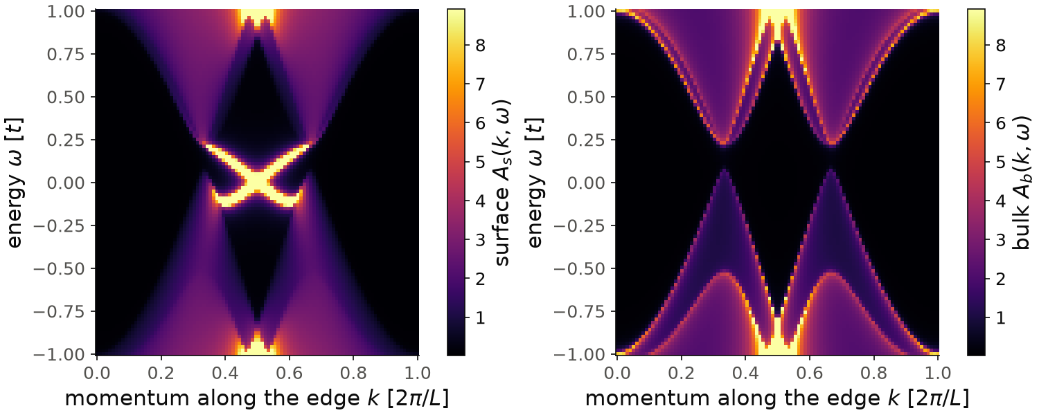
\(k\) is the momentum along the edge, in units of \(2\pi/L\) with \(L\) the period of the edge. In the bulk (right), the bands have a gap at \(k=1/3\) and \(k=2/3\), the projections of K and K'. The gap goes from \(0.075t\) to \(0.22t\), the same as in the band structure of the two-dimensional crystal: the spin-orbit coupling opens it and the Rashba coupling makes it smaller. At the surface (left), two bright lines cross this gap and meet at \(k=1/2\) near \(\omega=0\). These are the helical edge states, which cross at the time-reversal invariant momentum. The color scale is the same in the two panels and saturates on the edge states.

Code of this figure (documentation/figures/spectral_surface.py)

import numpy as np
import style
from pyqula import geometry

g = geometry.honeycomb_lattice() # create honeycomb lattice
h = g.get_hamiltonian() # create hamiltonian of the system
h.add_soc(0.05) # Kane-Mele spin-orbit coupling opens a topological gap
h.add_rashba(0.1) # break z-mirror symmetry to expose the edge states
(k,e,ds,db) = h.get_surface_kdos(delta=1e-2) # surface and bulk spectral functions

nk, ne = len(np.unique(k)), len(np.unique(e))
(k,e,ds,db) = [a.reshape(nk,ne) for a in (k,e,ds,db)] # k is the outer index

def draw(ax, c):
    for a, d, name in zip(ax, [ds, db], ["surface $A_s$", "bulk $A_b$"]):
        im = a.pcolormesh(k, e, d, cmap=c.cmap, shading="auto", vmax=np.percentile(ds,98))
        style.colorbar(im, a, name+r"$(k,\omega)$")
        a.set_xlabel(r"momentum along the edge $k$ [$2\pi/L$]")
        a.set_ylabel(r"energy $\omega$ [$t$]")

style.save(draw, "spectral_surface", npanels=2)

See examples/readme_examples/surface_2dTI/main.py for a runnable script, and jupyter-notebooks/functionalities/spectral_functions/02_surface_spectral_semiinfinite.ipynb for an executed notebook.

The surface density of states, integrated over \(k\), is dos.surface_dos(h,...), which returns the surface and bulk densities of states at a set of energies, with the same normalization as \(A_s\) (without the \(1/\pi\)). It also takes an operator=, for example to get the spin-resolved surface density of states of a magnet. An operator that depends on momentum, such as "valley", is not accepted, because the Green's function has already been summed over \(k\). The same decimation of a semi-infinite lead is used in Quantum transport.