Band unfolding

In this page we see how the band structure of a supercell is folded into its smaller Brillouin zone, and how to unfold it back to the Brillouin zone of the primitive cell, with operator="unfold".

Folding and unfolding

A supercell does not change the physics, but it changes how the bands are drawn. A supercell of \(N_c\) primitive cells has a Brillouin zone \(N_c\) times smaller, and the bands of the primitive cell fold into it, so the supercell has \(N_c\) times more bands, all of them copies of the same dispersion. We use a supercell when there is a reason for it: a defect, a moire pattern, a charge density wave. To compare with ARPES, we want the opposite operation. ARPES measures the spectral weight on the Bloch states of the primitive cell, so when the perturbation is weak it sees the bands of the primitive cell, and only weak shadows of the folded copies.

Let \(\mathbf R\) be the positions of the \(N_c\) copies of the primitive cell inside the supercell, and \(\alpha\) the orbitals of the primitive cell. The Bloch state of the primitive cell with momentum \(\mathbf k\) is

\[ |\mathbf k,\alpha\rangle = \sum_{\mathbf R} e^{i\mathbf k\cdot\mathbf R}\,|\mathbf R,\alpha\rangle , \]

and the unfolded spectral function is the spectral weight on these states,

\[ A(\mathbf k,\omega) = \sum_\alpha \langle \mathbf k,\alpha|\,\delta(\omega-H)\,|\mathbf k,\alpha\rangle , \]

where \(H\) is the Hamiltonian of the supercell at the momentum of the supercell that corresponds to \(\mathbf k\). The Bloch states are not normalized, so for a supercell without any perturbation \(A(\mathbf k,\omega)\) is \(N_c\) times the spectral function of the primitive cell. In pyqula this projection is the operator "unfold". It can be given to the observables that are resolved in momentum, h.get_bands(), h.get_kdos_bands() and h.get_multi_fermi_surface(). The supercell must be built with store_primal=True, so that the primitive cell is known:

from pyqula import geometry
import numpy as np
g = geometry.honeycomb_lattice() # primitive geometry
n = 3
gs = g.get_supercell(n,store_primal=True) # supercell, keeping the primitive cell info
h = gs.get_hamiltonian() # Hamiltonian of the supercell
kpath = gs.get_unfolded_kpath(nk=200) # primitive k-path, in supercell coordinates
(k,e,d) = h.get_kdos_bands(operator="unfold",delta=1e-1,kpath=kpath) # unfolded weight

gs.get_unfolded_kpath() gives the k-path of the primitive cell, written in the coordinates of the supercell (see Which k-path to unfold along below). d is the unfolded weight at each (k,e). A scatter plot of k,e colored by d gives the band structure of the primitive cell: the folded copies that a plain h.get_bands() of the supercell shows have no weight, and the Dirac cones of the honeycomb lattice appear at K, where they belong. To unfold a constant-energy cut, give the same operator to h.get_multi_fermi_surface() (see Spectral functions).

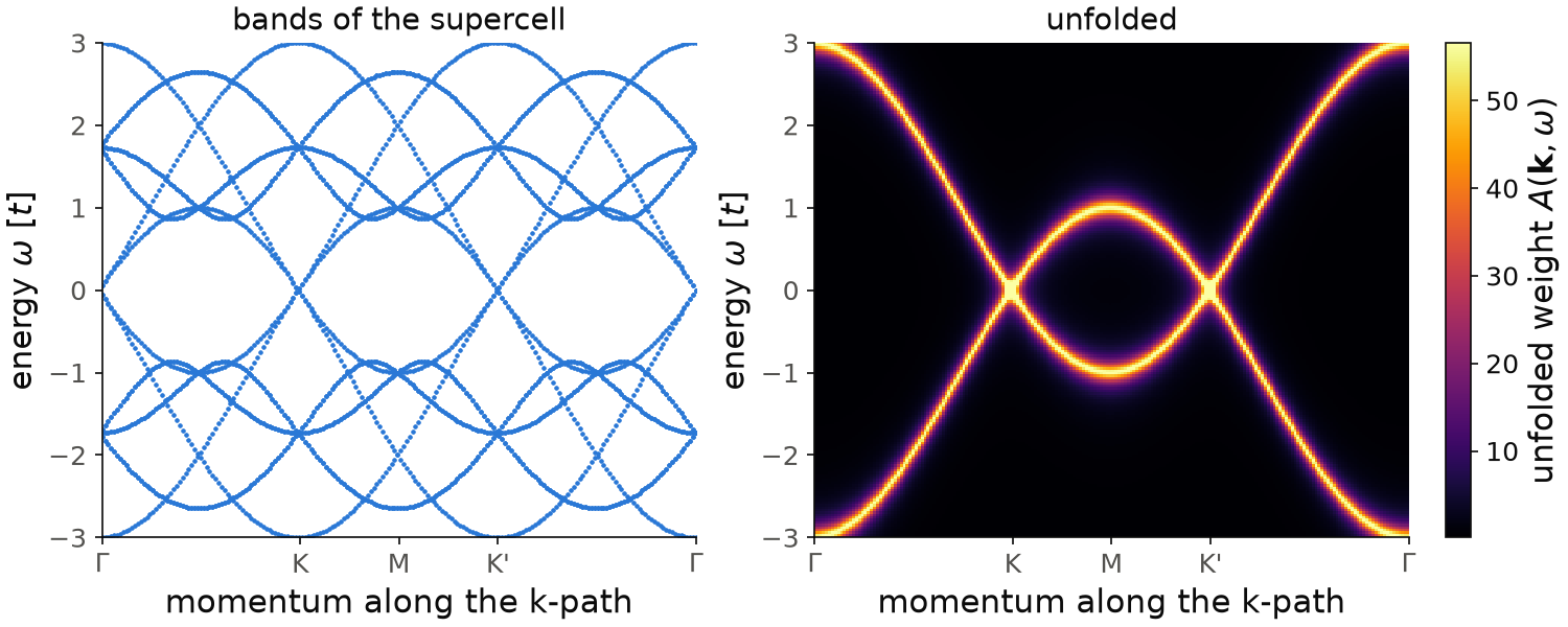
On the left, h.get_bands(kpath=kpath) of the supercell along the same path, with nine times more bands. In a \(3\times 3\) supercell K folds onto \(\Gamma\), so the folded bands also touch at zero energy at \(\Gamma\). On the right, the unfolded weight shows only the two bands of the primitive cell, from \(-3t\) to \(3t\), with the Dirac points at K and K'. The weight under each band is nine times the one of the primitive cell, since the Bloch states are not normalized.

Code of this figure (documentation/figures/unfolding_honeycomb.py)

import style
from pyqula import geometry
import numpy as np
g = geometry.honeycomb_lattice() # primitive geometry
n = 3
gs = g.get_supercell(n,store_primal=True) # supercell, keeping the primitive cell info
h = gs.get_hamiltonian() # Hamiltonian of the supercell
kpath = gs.get_unfolded_kpath(nk=200) # primitive k-path, in supercell coordinates
(k,e,d) = h.get_kdos_bands(operator="unfold",delta=1e-1,kpath=kpath) # unfolded weight
(k0,e0) = h.get_bands(kpath=kpath) # the folded bands, on the same path

nk, ne = len(np.unique(k)), len(np.unique(e)) # k is the outer index
(k,e,d) = [a.reshape(nk,ne) for a in (k,e,d)]

def draw(ax, c):
    ax[0].scatter(k0/k0.max(), e0, s=1, color=c.blue)
    ax[0].set_title("bands of the supercell")
    im = ax[1].pcolormesh(k/k.max(), e, d, cmap=c.cmap, shading="auto", vmax=np.percentile(d,99))
    style.colorbar(im, ax[1], r"unfolded weight $A(\mathbf{k},\omega)$")
    ax[1].set_title("unfolded")
    for a in ax:
        a.set_xticks([0,1/3,1/2,2/3,1]) # the default path
        a.set_xticklabels([r"$\Gamma$", "K", "M", "K'", r"$\Gamma$"])
        a.set_xlim(0, 1)
        a.set_ylim(e.min(), e.max())
        a.set_xlabel("momentum along the k-path")
        a.set_ylabel(r"energy $\omega$ [$t$]")

style.save(draw, "unfolding_honeycomb", npanels=2)

See examples/2d/unfolding/main.py, examples/1d/unfolding/main.py and examples/readme_examples/unfolding_FS/main.py for runnable scripts, and jupyter-notebooks/functionalities/single_particle_hamiltonians/08_unfolding_supercells.ipynb for an executed notebook.

Unfolding also works when sites are removed from the supercell, for example a vacancy or a flake cut out of the supercell, with gs = gs.remove([...]) before gs.get_hamiltonian(). Each remaining site is matched to its copy of the primitive cell by its position, so the sites must not be moved (for example with gs.center() or a relaxation) between gs.remove(...) and gs.get_hamiltonian(). If they are moved, the unfolding raises a ValueError.

General supercells

A supercell does not need to be \(n\times n\). Its lattice vectors can be any integer combinations of the primitive ones, \(\mathbf A = M\mathbf a\), with \(M\) a 3x3 integer matrix, and \(N_c=|\det M|\). Give \(M\) to g.get_supercell(), and the unfolding works in the same way:

from pyqula import geometry
g = geometry.honeycomb_lattice() # primitive geometry
M = [[2,1,0],[0,1,0],[0,0,1]] # non-diagonal supercell matrix, det(M)=2
gs = g.get_supercell(M,store_primal=True) # supercell, keeping the primitive cell info
h = gs.get_hamiltonian() # Hamiltonian of the supercell
kpath = gs.get_unfolded_kpath(nk=200) # primitive k-path, in supercell coordinates
(k,e,d) = h.get_kdos_bands(operator="unfold",delta=1e-1,kpath=kpath) # unfolded weight

Nothing in the formula above depends on the dimension, so it works in the same way for a chain, a two-dimensional lattice and a three-dimensional crystal:

from pyqula import geometry
g = geometry.cubic_lattice() # three dimensional primitive geometry
gs = g.get_supercell([2,2,2],store_primal=True) # supercell, keeping the primitive cell info
h = gs.get_hamiltonian() # Hamiltonian of the supercell
kpath = gs.get_unfolded_kpath(nk=200) # primitive k-path, in supercell coordinates
(k,e,d) = h.get_bands(operator="unfold",kpath=kpath) # unfolded band structure

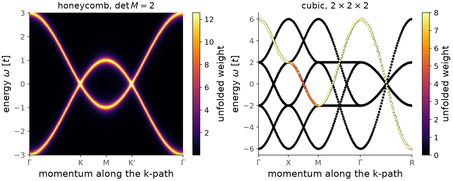
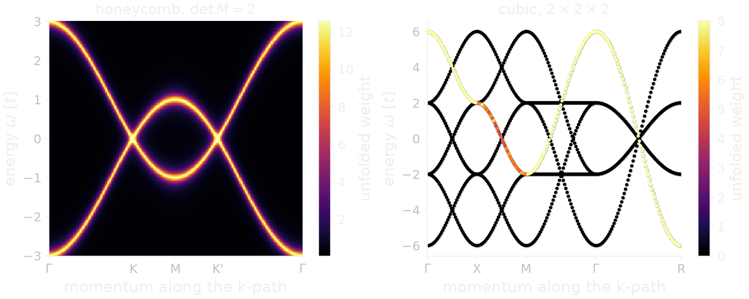
On the left, the non-diagonal supercell with \(\det M=2\) unfolds to the same two bands of the honeycomb lattice as the \(3\times 3\) one above. On the right, the \(2\times2\times2\) supercell of the cubic lattice has eight bands, and the color is the unfolded weight of each state. One band has the full weight \(8=N_c\): it goes from \(6t\) at \(\Gamma\) to \(2t\) at X, \(-2t\) at M, back to \(6t\) at \(\Gamma\) and to \(-6t\) at R, which is the band \(2t(\cos k_x+\cos k_y+\cos k_z)\) of the primitive cell. The other bands are the folded copies, with zero weight. Between X and M the band is degenerate with a folded copy, and the weight is shared between the two.

Code of this figure (documentation/figures/unfolding_general.py)

import numpy as np
import style
from pyqula import geometry

# honeycomb lattice, non-diagonal supercell
g = geometry.honeycomb_lattice() # primitive geometry
M = [[2,1,0],[0,1,0],[0,0,1]] # non-diagonal supercell matrix, det(M)=2
gs = g.get_supercell(M,store_primal=True) # supercell, keeping the primitive cell info
h = gs.get_hamiltonian() # Hamiltonian of the supercell
kpath = gs.get_unfolded_kpath(nk=200) # primitive k-path, in supercell coordinates
(k,e,d) = h.get_kdos_bands(operator="unfold",delta=1e-1,kpath=kpath) # unfolded weight

# cubic lattice, 2 x 2 x 2 supercell
g = geometry.cubic_lattice() # three dimensional primitive geometry
gs = g.get_supercell([2,2,2],store_primal=True) # supercell, keeping the primitive cell info
h = gs.get_hamiltonian() # Hamiltonian of the supercell
kpath = gs.get_unfolded_kpath(nk=200) # primitive k-path, in supercell coordinates
(k3,e3,d3) = h.get_bands(operator="unfold",kpath=kpath) # unfolded band structure

nk, ne = len(np.unique(k)), len(np.unique(e)) # k is the outer index
(k,e,d) = [a.reshape(nk,ne) for a in (k,e,d)]
i = np.argsort(d3) # draw the states with weight on top
ticks = np.cumsum([0,.5,.5,np.sqrt(.5),np.sqrt(.75)]) # lengths of the segments of the cubic path

def draw(ax, c):
    im = ax[0].pcolormesh(k/k.max(), e, d, cmap=c.cmap, shading="auto", vmax=np.percentile(d,99))
    style.colorbar(im, ax[0], "unfolded weight")
    ax[0].set_xticks([0,1/3,1/2,2/3,1]) # the default path
    ax[0].set_xticklabels([r"$\Gamma$", "K", "M", "K'", r"$\Gamma$"])
    ax[0].set_title(r"honeycomb, $\det M=2$")
    ax[1].scatter(k3/k3.max(), e3, s=8, color=c.ink2) # outline, so that zero weight stays visible
    sc = ax[1].scatter(k3[i]/k3.max(), e3[i], c=d3[i], s=4, cmap=c.cmap, vmin=0)
    style.colorbar(sc, ax[1], "unfolded weight")
    ax[1].set_xticks(ticks/ticks[-1])
    ax[1].set_xticklabels([r"$\Gamma$", "X", "M", r"$\Gamma$", "R"])
    ax[1].set_title(r"cubic, $2\times2\times2$")
    for a in ax:
        a.set_xlim(0, 1)
        a.set_xlabel("momentum along the k-path")
        a.set_ylabel(r"energy $\omega$ [$t$]")

style.save(draw, "unfolding_general", npanels=2)

See examples/2d/unfolding_nonorthogonal/main.py for a runnable script with a defect in a non-diagonal supercell, and examples/3d/unfolding/main.py for the three-dimensional case.

A supercell can also be asked for by its size only. The most common case is the \(\sqrt3\times\sqrt3\) supercell of a triangular or honeycomb lattice, the unit cell of a charge order with three sublattices:

from pyqula import geometry
import numpy as np
g = geometry.triangular_lattice() # primitive geometry
gs = g.get_supercell(np.sqrt(3),store_primal=True) # sqrt(3) x sqrt(3) supercell

A non-integer size \(s\) means a cell \(s^2\) times larger in area, here three primitive cells. g.get_supercell() returns the most compact cell of this size. For the triangular lattice it has \(|\mathbf A_1|=|\mathbf A_2|=\sqrt3\) in units of the lattice constant, with 60 degrees between them, and it is rotated so that \(\mathbf A_1\) is along \(x\). The matrix that was used is gs.supercell_matrix. To choose the matrix and the orientation yourself, give an explicit \(M\).

Which k-path to unfold along

The unfolded bands must be drawn along a path of the Brillouin zone of the primitive cell. A momentum \(\mathbf k_0\) of the primitive cell corresponds to the momentum \(\mathbf k = M\mathbf k_0\) in the reduced coordinates of the supercell. For an \(n\times n\) supercell this is the primitive path multiplied by \(n\). For the \(\sqrt3\times\sqrt3\) supercell it is also a rotation, which no multiplication by a number can give. gs.get_unfolded_kpath() returns the right path for any supercell. Here we add a three-sublattice charge order to the \(\sqrt3\times\sqrt3\) supercell of the triangular lattice:

from pyqula import geometry
import numpy as np
g = geometry.triangular_lattice() # primitive geometry
gs = g.get_supercell(np.sqrt(3),store_primal=True) # sqrt(3) x sqrt(3) supercell
h = gs.get_hamiltonian() # Hamiltonian of the supercell
fons = lambda r: (np.sum((r - gs.r[0])**2)<1e-2)*0.6 # onsite in one of the three sites
h.add_onsite(fons) # three-sublattice charge order
kpath = gs.get_unfolded_kpath(nk=200) # primitive k-path, in supercell coordinates
(k,e,d) = h.get_kdos_bands(operator="unfold",delta=1e-1,kpath=kpath) # unfolded weight

The k-points are in the reduced coordinates of the supercell, which is what kpath= takes. gs.get_unfolded_kpath() takes the same arguments as g.get_kpath(), so the high-symmetry points can be named, gs.get_unfolded_kpath(["G","K","M","G"],nk=400), and they are the points of the primitive cell. In the plot of k,e colored by d you see the single band of the triangular lattice along \(\Gamma\)-K-M-K'-\(\Gamma\), with a gap opened at K by the charge order, and a weak shadow band, the folded copy, with the small weight that the modulation gives it. Along the k-path of the supercell, gs.get_kpath(), the same calculation goes along a path of the primitive Brillouin zone that has no special meaning. See examples/2d/unfolding_sqrt3/main.py for a runnable script.

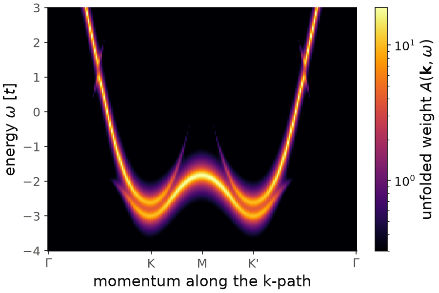
For the figure we take energies=np.linspace(-4,3,300), since the default window starts at \(-3\), the bottom of the band. The color scale is logarithmic, so that the weak shadow band is visible. At K and K' the charge order splits the bottom of the band into two states, at \(-3.0t\) and \(-2.6t\). The shadow band is the faint line that rises from M up to about \(-0.5t\), and it crosses the main band at about \(1.3t\), once between \(\Gamma\) and K and once between K' and \(\Gamma\), where a small gap opens.

Code of this figure (documentation/figures/unfolding_sqrt3.py)

import style
from pyqula import geometry
import numpy as np
g = geometry.triangular_lattice() # primitive geometry
gs = g.get_supercell(np.sqrt(3),store_primal=True) # sqrt(3) x sqrt(3) supercell
h = gs.get_hamiltonian() # Hamiltonian of the supercell
fons = lambda r: (np.sum((r - gs.r[0])**2)<1e-2)*0.6 # onsite in one of the three sites
h.add_onsite(fons) # three-sublattice charge order
kpath = gs.get_unfolded_kpath(nk=200) # primitive k-path, in supercell coordinates
(k,e,d) = h.get_kdos_bands(operator="unfold",delta=1e-1,kpath=kpath,
        energies=np.linspace(-4,3,300)) # unfolded weight, down to below the band

nk, ne = len(np.unique(k)), len(np.unique(e)) # k is the outer index
(k,e,d) = [a.reshape(nk,ne) for a in (k,e,d)]

def draw(ax, c):
    im = ax.pcolormesh(k/k.max(), e, d, cmap=c.cmap, shading="auto",
            norm="log", vmin=0.3, vmax=d.max()) # a log scale shows the weak shadow band
    style.colorbar(im, ax, r"unfolded weight $A(\mathbf{k},\omega)$")
    ax.set_xticks([0,1/3,1/2,2/3,1]) # the default path
    ax.set_xticklabels([r"$\Gamma$", "K", "M", "K'", r"$\Gamma$"])
    ax.set_xlabel("momentum along the k-path")
    ax.set_ylabel(r"energy $\omega$ [$t$]")

style.save(draw, "unfolding_sqrt3")

Unfolding a large supercell with the kernel polynomial method

The cases where unfolding matters most, a moire pattern or a disordered region, have the largest supercells, and there diagonalizing the Hamiltonian at each k-point is too expensive. With h.get_kdos_bands(operator="unfold",mode="KPM"), each term \(\langle \mathbf k,\alpha|\delta(\omega-H)|\mathbf k,\alpha\rangle\) of the formula above is computed with a Chebyshev expansion (see Kernel polynomial method), started from the Bloch state \(|\mathbf k,\alpha\rangle\) itself. So no random vectors are needed, and the result has no statistical noise:

import numpy as np
from pyqula import geometry
from pyqula import potentials
g0 = geometry.triangular_lattice() # primitive geometry
g = g0.get_supercell(12,store_primal=True) # supercell of 144 primitive cells
h = g.get_hamiltonian() # Hamiltonian of the supercell
fmoire = potentials.commensurate_potential(g,n=3,minmax=[0,1]) # moire potential
h.add_onsite(fmoire) # onsite energy following the moire
kpath = g.get_unfolded_kpath(nk=300) # primitive k-path, in supercell coordinates
(k,e,d) = h.get_kdos_bands(operator="unfold",mode="KPM",delta=5e-2,kpath=kpath,
        energies=np.linspace(-3,-1,200)) # unfolded weight, with the KPM

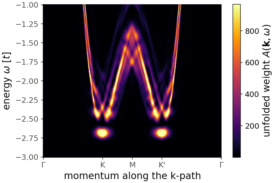
The moire potential splits the bottom of the band into minibands. The lowest state is at K and K', at about \(-2.7t\), above the \(-3t\) of the clean lattice because the potential is positive. It is separated by a gap from the next minibands, which start at about \(-2.5t\). Around M you see several copies of the band, shifted by the moire wavevectors, each one with a part of the weight.

The k-path needs more points than for a band structure. Between two neighboring k-points a steep band moves in energy, and if this step is larger than delta the band shows up as a row of separate dots. With nk=100 the steep branches of the map break into such dots. With nk=300 they are continuous lines, and the map does not change any more when we go to nk=600. There is no other convergence parameter: the expansion has no random vectors, and the number of polynomials follows from delta.

Code of this figure (documentation/figures/unfolding_kpm.py)

import numpy as np
import style
from pyqula import geometry
from pyqula import potentials
g0 = geometry.triangular_lattice() # primitive geometry
g = g0.get_supercell(12,store_primal=True) # supercell of 144 primitive cells
h = g.get_hamiltonian() # Hamiltonian of the supercell
fmoire = potentials.commensurate_potential(g,n=3,minmax=[0,1]) # moire potential
h.add_onsite(fmoire) # onsite energy following the moire
kpath = g.get_unfolded_kpath(nk=300) # primitive k-path, in supercell coordinates
(k,e,d) = h.get_kdos_bands(operator="unfold",mode="KPM",delta=5e-2,kpath=kpath,
        energies=np.linspace(-3,-1,200)) # unfolded weight, with the KPM

nk, ne = len(np.unique(k)), len(np.unique(e)) # k is the outer index
(k,e,d) = [a.reshape(nk,ne) for a in (k,e,d)]

def draw(ax, c):
    im = ax.pcolormesh(k/k.max(), e, d, cmap=c.cmap, shading="auto", vmax=np.percentile(d,99))
    style.colorbar(im, ax, r"unfolded weight $A(\mathbf{k},\omega)$")
    ax.set_xticks([0,1/3,1/2,2/3,1]) # the default path
    ax.set_xticklabels([r"$\Gamma$", "K", "M", "K'", r"$\Gamma$"])
    ax.set_xlabel("momentum along the k-path")
    ax.set_ylabel(r"energy $\omega$ [$t$]")

style.save(draw, "unfolding_kpm")

The output is the same as with mode="ED", with the same weight under each band. Only the line shape is different: the Chebyshev expansion broadens each band with its kernel, with a number of polynomials set by delta, and not with a Lorentzian. The cost of each k-point grows linearly with the number of sites of the supercell, not with its cube, so supercells with thousands of sites are possible. A smaller delta needs proportionally more polynomials.