Topological invariants

A topological insulator has a gap in the bulk and states at the edges that no perturbation can remove, as long as the gap stays open. A topological invariant is an integer computed from the occupied bands over the whole Brillouin zone. An integer cannot change continuously, so the only way to change it is to close the gap. This is why the edge states it counts are protected. In this page we see the Chern number, the \(Z_2\) invariant, the spin and mirror Chern numbers, the quadrupole moment, the three-dimensional \(Z_2\) indices and the one-dimensional invariants.

Chern number

The Chern number is the invariant of a two-dimensional insulator with broken time-reversal symmetry. It is computed with h.get_chern(). For the occupied Bloch states \(|u_n(\mathbf k)\rangle\), the Berry connection is \(\mathbf A(\mathbf k) = i\sum_n \langle u_n|\nabla_{\mathbf k} u_n\rangle\), the Berry curvature is \(\Omega(\mathbf k) = \partial_{k_x}A_y - \partial_{k_y}A_x\), and the Chern number is

\[ C = \frac{1}{2\pi} \int_{\rm BZ} \Omega (\mathbf k)\, d^2 \mathbf k , \]

the total Berry flux of the occupied bands through the Brillouin zone, in units of \(2\pi\). The occupied bands are those with energy below zero, the Fermi energy. \(C\) is an integer. It is the Hall conductivity of the insulator in units of \(e^2/h\), and it is the number of chiral states that cross the gap at each edge, so it is measured in a Hall experiment.

We take the Haldane model: a honeycomb lattice with a complex second-neighbor hopping, which breaks time-reversal symmetry and opens a topological gap at the Dirac points.

from pyqula import geometry
from pyqula import kdos
g = geometry.honeycomb_lattice() # create honeycomb lattice
h = g.get_hamiltonian() # create hamiltonian of the system
h.add_haldane(0.05) # Add Haldane coupling
C = h.get_chern() # Chern number

The result is \(C=2\). The Hamiltonian is spinful by default, and the Haldane term is the same for both spins, so each spin gives one. The same model with has_spin=False gives \(C=1\).

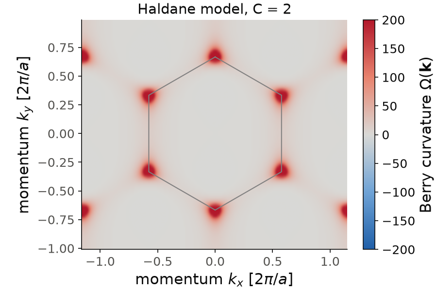
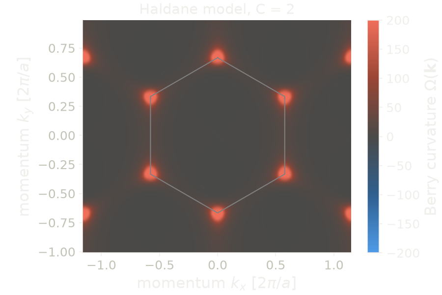
The map is the Berry curvature \(\Omega(\mathbf k)\) of this snippet, computed with h.get_berry_curvature(nk=100). It covers a rectangle of momenta centered at \(\Gamma\), from \(-0.577\) to \(0.577\) in \(k_x\) and from \(-1\) to \(1\) in \(k_y\), and this rectangle holds exactly two Brillouin zones. The curvature is periodic, so the figure shows the map repeated once along \(k_x\), with one zone drawn as the gray hexagon. The curvature is in the units of the reduced Brillouin zone, whose area is one. It is concentrated at the six corners of the zone, the K and K' points, where the gap is smallest, from \(-0.225\) to \(0.225\). Its peak is about \(620\), so the color scale is cut at \(200\) to show the tails. The curvature has the same sign at K and at K', so the two valleys add up instead of cancelling. These sharp peaks are what the k-mesh has to resolve.

Because the map holds a whole number of zones, the Chern number comes back from it as the mean of the curvature divided by \(2\pi\). Here np.mean(b)/(2*np.pi) is \(2.000\), the same as h.get_chern(). The window is chosen in the same way for every two-dimensional lattice. For a square lattice it is one zone, a square of side \(|\mathbf b_1|\), and for a hexagonal lattice it is the rectangle of two zones of the figure, of sides \(|\mathbf b_1|\) and \(\sqrt{3}|\mathbf b_1|\). A lattice without such a rectangle, for example an oblique one, gets the parallelogram spanned by its two reciprocal lattice vectors, one zone, and then the points of the map are not on a rectangular grid. With reciprocal=False the map uses the reduced momenta from \(-1\) to \(1\), four zones, and the mean gives the Chern number too.

Code of this figure (documentation/figures/topology_chern.py)

import numpy as np
import style
from pyqula import geometry
from pyqula import kdos
g = geometry.honeycomb_lattice() # create honeycomb lattice
h = g.get_hamiltonian() # create hamiltonian of the system
h.add_haldane(0.05) # Add Haldane coupling
C = h.get_chern() # Chern number
nk = 100 # k-points per direction
(kx,ky,b) = h.get_berry_curvature(nk=nk) # Berry curvature, a window of two zones
print("mean/(2 pi) =",np.mean(b)/(2*np.pi)) # the Chern number
b = b.reshape(nk,nk).T # as an image, ky along the rows
(Lx,Ly) = (-2*kx.min(),-2*ky.min()) # the window is centered at Gamma
b = np.concatenate([b[:,nk//2:],b,b[:,:nk//2]],axis=1) # periodic, shown twice as wide
(dx,dy) = (Lx/nk/2,Ly/nk/2) # half a pixel
phi = np.pi/2 + np.pi/3*np.arange(7) # corners of the Brillouin zone, the K points

def draw(ax, c):
    im = ax.imshow(b, origin="lower", extent=[-Lx-dx,Lx-dx,-Ly/2-dy,Ly/2-dy], cmap=c.diverging,
                   vmin=-200, vmax=200, interpolation="bicubic")
    ax.plot(2/3*np.cos(phi), 2/3*np.sin(phi), color="gray", lw=1)
    style.colorbar(im, ax, r"Berry curvature $\Omega(\mathbf{k})$")
    ax.set_xlabel(r"momentum $k_x$ [$2\pi/a$]")
    ax.set_ylabel(r"momentum $k_y$ [$2\pi/a$]")
    ax.set_title(f"Haldane model, C = {C:.0f}")

style.save(draw, "topology_chern")

The integral is a sum over a k-mesh of nk points per direction, ten by default. The default sum counts the Berry phase around each small plaquette of the mesh, so it gives an integer at every nk. But the integer is only the right one if the mesh resolves the Berry curvature. Close to a gap closing, the curvature is sharply peaked near the gap minimum, and then nk must be larger.

Keywords:

• nk: number of k-points per direction of the mesh.
• operator: weight the curvature with an operator, for example a spin or a valley. This gives a spin or a valley Chern number (see Operators).
• integration: how the integral is done, "grid" (default), "qtci" or "wannier", explained below.

h.get_berry_curvature() returns the curvature \(\Omega(\mathbf k)\) itself, as a map over the Brillouin zone. h.get_berry_curvature_path() returns it along a k-path, by default the k-path of h.get_bands(), so that the peaks of the curvature can be put next to the band structure.

See examples/2d/chern/main.py (a Chern insulator from Rashba coupling and an exchange field), examples/2d/haldane_model/main.py and examples/2d/valley_chern/main.py for runnable scripts, and jupyter-notebooks/functionalities/topological_characterization/01_chern_z2.ipynb and 02_operator_resolved_chern.ipynb for the curvature maps.

Adaptive integration with tensor cross interpolation

With integration="qtci", the Brillouin-zone integral is done by quantics tensor cross interpolation. The integrand is learned on an adaptive grid, with more points where it changes fast, and then integrated with a quadrature rule. The number of evaluations grows roughly as the logarithm of the resolution, instead of as nk squared.

from pyqula import geometry
g = geometry.honeycomb_lattice()
h = g.get_hamiltonian()
h.add_haldane(0.05)
C = h.get_chern(integration="qtci",nk=20) # tensor-cross-interpolated BZ integral

Use it only for a smooth Berry curvature, so for a large gap. There it gives the integer to between \(10^{-5}\) and \(10^{-9}\) with far fewer evaluations than a dense mesh. For a small gap it is the wrong choice: the Haldane model above, with its small gap, gives \(C=2.015\) at nk=20, and the error grows with nk, because the quadrature nodes miss the peak of the curvature. For a small gap, use the default grid, which is exactly quantized.

The same method can replace the k-mesh sum of the density matrix in a mean-field calculation (see Mean-field Hubbard models):

from pyqula import geometry
g = geometry.honeycomb_lattice()
h = g.get_hamiltonian()
hscf,e = h.get_mean_field_hamiltonian(U=2.0,filling=0.5,mf="antiferro",
        nk=8,maxerror=1e-4,return_total_energy=True,integration="qtci")

For an insulator, "qtci" and the k-mesh sum agree. For a metal, the density matrix has a step at the Fermi surface, and a quadrature rule converges slowly on a step. For an attractive \(U=-2\) on the square lattice at filling=0.3, the pairing gap is 16% too small at nk=8 and within 3% at nk=16. This mode works for two-dimensional Hamiltonians only, and in two dimensions it is not cheaper than the k-mesh sum. See examples/2d/chern_qtci/main.py and examples/2d/mean_field_qtci/main.py.

Winding of the hybrid Wannier centers

With integration="wannier", the Chern number is obtained without the Berry curvature. We fix the momentum \(k_2\) along the second reciprocal direction. The system is then a one-dimensional chain along the first direction. For this chain we compute the Wilson loop of the occupied bands, the product of the overlaps \(\langle u_n(\mathbf k)|u_m(\mathbf k+\delta \mathbf k)\rangle\) around the closed loop in \(k_1\). The phases of its eigenvalues are the positions of the hybrid Wannier centers: the centers of charge of states that are localized along the first direction and extended along the second. When \(k_2\) goes once around the Brillouin zone, the sum of the centers moves by \(-C\) lattice constants, with \(C\) the Chern number of h.get_chern(). So for \(C=2\) the centers move by two lattice constants towards negative positions. The Chern number is the charge pumped across the unit cell in one cycle, and its sign is the direction of the pumping.

from pyqula import geometry
g = geometry.honeycomb_lattice() # create honeycomb lattice
h = g.get_hamiltonian() # create hamiltonian of the system
h.add_haldane(0.05) # Add Haldane coupling
C = h.get_chern(integration="wannier") # winding of the hybrid Wannier centers

The result is \(C=2\), as with the grid. The winding is always an integer. It is the right integer if the sum of the centers moves by less than half a lattice constant between two consecutive values of \(k_2\). There are nt values of \(k_2\) (100 by default) and nk k-points along each Wilson loop (30 by default). The centers move fastest where the gap is smallest, so the gap decides how large nt must be: with a Haldane coupling of \(0.02\), nt=20 gives 0 and nt=50 gives 2.

The flow of the centers, the curve one plots to see the pumping, is returned by topology.z2_wannier_centers(h,full=True). Its first row is \(k_2\), and there is one row per occupied band after it, each center given as the phase \(2\pi x\) of its fractional coordinate \(x\) along the loop.

• loop, pump: the two reciprocal directions, of the Wilson loop and of the pumping.
• gauge="atomic": put each orbital at its real position in the cell, instead of at the origin of the cell. The windings do not change, but the centers move to where the charge really is. Use it when the positions themselves matter, for example for a polarization.

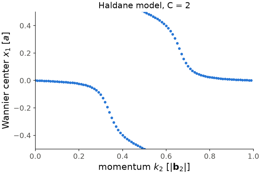
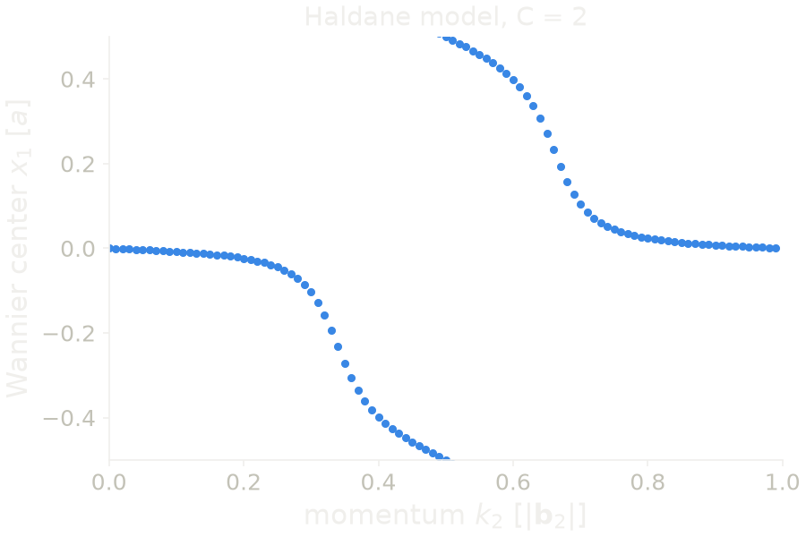
The figure shows this flow for the Haldane model of the snippet, with the center written as \(x_1\), in units of the lattice constant. The two spins have the same center, so the two rows lie on top of each other. At \(k_2=0\) the center is at \(0\). It moves slowly, then fast near \(k_2=1/3\), where the gap is smallest, and reaches the border of the cell, \(x_1=-1/2\), at \(k_2=1/2\). It comes back in at \(+1/2\) and goes back to \(0\) at \(k_2=1\). So in one cycle each spin moves by one lattice constant towards negative \(x_1\). The two spins together move by \(-2\) lattice constants, so \(C=2\). The plot repeats the center at \(x_1\pm1\), so that the line is continuous across the border of the cell.

Code of this figure (documentation/figures/topology_wannier.py)

import numpy as np
import style
from pyqula import geometry
from pyqula import topology
g = geometry.honeycomb_lattice() # create honeycomb lattice
h = g.get_hamiltonian() # create hamiltonian of the system
h.add_haldane(0.05) # Add Haldane coupling
C = h.get_chern(integration="wannier") # winding of the hybrid Wannier centers
w = topology.z2_wannier_centers(h,full=True) # flow of the centers over the whole BZ
k2 = w[0] # momentum along the pumping direction
x = np.array(w[1:])/(2*np.pi) # centers, in units of the lattice constant

def draw(ax, c):
    for xi in x: # one row per occupied band, the two spins on top of each other
        for shift in [-1,0,1]: # periodic copies, so that the winding is visible
            ax.scatter(k2, xi+shift, s=10, color=c.blue)
    ax.set_ylim(-0.5, 0.5)
    ax.set_xlim(0, 1)
    ax.set_xlabel(r"momentum $k_2$ [$|\mathbf{b}_2|$]")
    ax.set_ylabel(r"Wannier center $x_1$ [$a$]")
    ax.set_title(f"Haldane model, C = {C:.0f}")

style.save(draw, "topology_wannier")

See examples/2d/wannier_centers/main.py for a script that plots the flow.

Z2 invariant

With time-reversal symmetry the Chern number is zero. The invariant that remains is the \(Z_2\) index. It has two values: trivial, or quantum spin Hall insulator, with a helical pair of states at each edge. We compute it for the Kane-Mele model, a honeycomb lattice with intrinsic spin-orbit coupling, with topology.z2_invariant():

from pyqula import geometry
from pyqula import kdos
g = geometry.honeycomb_lattice() # create honeycomb lattice
h = g.get_hamiltonian() # create hamiltonian of the system
h.add_soc(0.05) # Add spin-orbit coupling
from pyqula import topology
z2 = topology.z2_invariant(h) # Z2 invariant

The result is a parity: \(-1\) for a topological insulator and \(+1\) for a trivial one. Here it is \(-1\). The honeycomb lattice gapped by a sublattice imbalance instead gives \(+1\). The invariant is the parity of the number of helical pairs at each edge. An odd number of Kramers pairs crossing the gap cannot be removed by any perturbation that keeps time-reversal symmetry, but an even number can. Two helical pairs can hybridize and open a gap.

It is computed from the flow of the hybrid Wannier centers over half of the Brillouin zone, from \(k_2=0\) to \(k_2=1/2\), the two time-reversal invariant lines. On this half, the Kramers partners either switch or come back to themselves, and the parity of the number of times the centers cross a fixed line tells which. The keywords are nk momenta along the loop and nt pumping steps, 60 each by default. h.add_soc() is the same term as h.add_kane_mele().

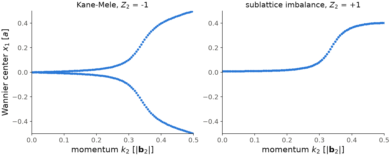
On the left is the flow of the Kane-Mele model of the snippet. On the right is the same lattice with a sublattice imbalance of \(0.2\) instead of the spin-orbit coupling, a trivial insulator. In the Kane-Mele model the two Kramers partners start together at \(x_1=0\) for \(k_2=0\). They separate, and at \(k_2=1/2\) they arrive at \(x_1=+1/2\) and \(x_1=-1/2\), which is the same point of the periodic cell. So each partner ends with a new partner: they have switched. In the trivial insulator the pair starts at \(x_1=0.008\) and ends at \(x_1=0.40\), still together. A horizontal line at any \(x_1\) is crossed once by the Kane-Mele flow, and an even number of times, zero or two, by the trivial one. This parity is the invariant.

Code of this figure (documentation/figures/topology_z2.py)

import numpy as np
import style
from pyqula import geometry
from pyqula import kdos
g = geometry.honeycomb_lattice() # create honeycomb lattice
h = g.get_hamiltonian() # create hamiltonian of the system
h.add_soc(0.05) # Add spin-orbit coupling
from pyqula import topology
z2 = topology.z2_invariant(h) # Z2 invariant
h0 = g.get_hamiltonian() # the trivial insulator, for comparison
h0.add_sublattice_imbalance(0.2) # gapped by a sublattice imbalance
z0 = topology.z2_invariant(h0) # Z2 invariant
w = topology.z2_wannier_centers(h) # flow of the centers over half of the BZ
w0 = topology.z2_wannier_centers(h0)

def draw(ax, c):
    for (axi,wi,zi,name) in zip(ax,[w,w0],[z2,z0],["Kane-Mele","sublattice imbalance"]):
        for xi in np.array(wi[1:])/(2*np.pi): # one row per occupied band
            axi.scatter(wi[0], xi, s=10, color=c.blue)
        axi.set_ylim(-0.5, 0.5)
        axi.set_xlim(0, 0.5)
        axi.set_xlabel(r"momentum $k_2$ [$|\mathbf{b}_2|$]")
        axi.set_title(f"{name}, $Z_2$ = {zi:+.0f}")
    ax[0].set_ylabel(r"Wannier center $x_1$ [$a$]")

style.save(draw, "topology_z2", npanels=2)

h.get_topological_invariant() chooses the invariant for you. In two dimensions it returns the \(Z_2\) invariant when the Hamiltonian is time-reversal symmetric, and the Chern number otherwise. In one dimension it returns the Berry phase, and in three dimensions the indices of the section on three dimensions below.

Time-reversal symmetric superconductors

The same index classifies a superconductor with time-reversal symmetry, a class DIII superconductor. Here it is the parity of the number of helical pairs of Majorana states at each edge, in-gap states that a tunneling probe at the edge would see. For a Bogoliubov-de Gennes (BdG) Hamiltonian, the invariant is computed from the negative-energy states. Time-reversal symmetry is checked up to a global phase of the pairing, since a uniform phase of the order parameter is only a gauge choice.

We take a helical p-wave superconductor on the square lattice. Spin up pairs as \(p_x-ip_y\) and spin down as \(p_x+ip_y\), so the two spins have opposite Chern numbers, and time reversal exchanges them.

import numpy as np
from pyqula import geometry
g = geometry.square_lattice() # square lattice, band between -4 and 4
h = g.get_hamiltonian() # spinful first-neighbor Hamiltonian
h.add_onsite(2.0) # chemical potential at -2, above the band bottom
def helical(r1,r2): # helical p-wave pairing, d-vector along the bond
    dr = r1-r2 # bond vector
    if abs(dr.dot(dr)-1.)>1e-4: return np.zeros((2,2)) # first neighbors only
    return 1j*np.array([[0.,dr[0]-1j*dr[1]],[dr[0]+1j*dr[1],0.]]) # i d.sigma
h.add_pairing(mode=helical,delta=0.3) # add the pairing, h is now a BdG Hamiltonian
z2 = h.get_topological_invariant() # Z2 invariant of the superconductor

The result is \(-1\) when the chemical potential is inside the band. It is \(+1\) when the chemical potential is below the band bottom, with h.add_onsite(5.0) instead of \(2\), because then there is no Fermi surface to pair. At half filling, h.add_onsite(0.0), the Fermi surface goes through the \(X\) points, where this pairing is zero, so the gap closes and the invariant is not defined.

Two remarks. First, the Kane-Mele insulator above gives \(+1\) once a small s-wave pairing is added, h.add_swave(0.01), although its normal state gives \(-1\). The Nambu doubling contains its helical edge twice, and the pairing gaps the two copies, so a quantum spin Hall insulator with s-wave pairing is a trivial superconductor. Second, the Chern number of each spin cannot be obtained with h.get_chern(operator="sz") in the helical superconductor. For a Nambu Hamiltonian "sz" is the operator \(\sigma_z\tau_0\), which this pairing does not conserve, and the weighted curvature integrates to zero. The operator that separates the two decoupled sectors is \(\sigma_z\tau_z\), Operator(np.diag([1.,-1.,-1.,1.])), and with it the weighted Chern number is \(C_\uparrow-C_\downarrow=-2\).

See examples/2d/z2_helical_superconductor/main.py for the invariant across the band, and examples/2d/z2_kane_mele/main.py and examples/2d/z2_transition/main.py (a transition driven by a sublattice imbalance) for the insulator.

Spin Chern number and mirror Chern number

The \(Z_2\) invariant needs time-reversal symmetry, and it is only a parity. Two other invariants count the helical pairs themselves, and they also exist when time reversal is broken: h.get_spin_chern() and h.get_mirror_chern(). Both are built in the same way. At every k-point, the occupied states are divided into two halves, by the sign of an operator projected on them. Each half has its own Chern number.

The simplest case is the spin. When \(s_z\) is conserved, the two halves are the two spin sectors, and the spin Chern number is

\[ C_s = \frac{C_+ - C_-}{2} , \]

half the difference of their Chern numbers. It counts the helical pairs at each edge, where the two spins move in opposite directions. When \(s_z\) is not conserved, for example with a Rashba coupling, the two halves are the eigenstates of \(P s_z P\), with \(P\) the projector on the occupied states. \(C_s\) is still an integer as long as the spectrum of \(P s_z P\) has a gap around zero, and the code checks this. With time-reversal symmetry, the parity of \(C_s\) is the \(Z_2\) invariant.

from pyqula import geometry
g = geometry.honeycomb_lattice() # create honeycomb lattice
h = g.get_hamiltonian() # create hamiltonian of the system
h.add_kane_mele(0.1) # Add spin-orbit coupling
h.add_rashba(0.1) # Add Rashba coupling, so that the spin is not conserved
Cs = h.get_spin_chern() # spin Chern number

The result is \(C_s=1\). Note that topology.spin_chern is a different quantity: the integral of the Berry curvature weighted by \(s_z\). It is \(C_\uparrow-C_\downarrow=2C_s\) when \(s_z\) is conserved, and it is not an integer here (2.097 with nk=24).

The mirror Chern number divides the occupied states by the eigenvalues \(\pm i\) of the mirror \(z\to -z\), which maps every momentum of a two-dimensional system to itself:

\[ C_M = \frac{C_{+i}-C_{-i}}{2} . \]

It is the invariant of a topological crystalline insulator, where the mirror, not time reversal, protects the edge states. The mirror is found from the geometry and the Hamiltonian, and the call raises an error when there is no mirror, for example with the Rashba coupling above, which breaks it.

from pyqula import geometry
g = geometry.honeycomb_lattice() # create honeycomb lattice
h = g.get_hamiltonian() # create hamiltonian of the system
h.add_kane_mele(0.1) # Add spin-orbit coupling
h.add_exchange([0.,0.,0.3]) # out-of-plane exchange: breaks time reversal, keeps the mirror
CM = h.get_mirror_chern() # mirror Chern number

The result is \(C_M=-1\). For a single layer the mirror is \(-i\sigma_z\), so \(C_M=-C_s\). It stays quantized with an out-of-plane exchange field, which keeps the mirror but breaks time reversal, so here the \(Z_2\) invariant is not even defined. For two coupled layers, the AA bilayer specialhamiltonian.multilayer_graphene(l=[0,0]) with the same spin-orbit coupling, we find \(C_s=2\) with a trivial \(Z_2\) invariant (two copies of the quantum spin Hall state), and \(C_M=0\), because the two mirror sectors have opposite Chern numbers.

• nk: number of k-points per direction of the mesh, 40 by default, for both calls.

See examples/2d/spin_mirror_chern/main.py for the two invariants as the Rashba coupling and the exchange field grow, and jupyter-notebooks/functionalities/topological_characterization/08_spin_mirror_chern.ipynb.

Quadrupole moment and the nested Wilson loop

A quadrupole insulator is a two-dimensional insulator with zero polarization and zero Chern number, but with a zero mode at each corner of a flake. STM would see these as peaks in the local density of states at the corners only. Its invariant is the quadrupole moment, computed with h.get_quadrupole_moment().

The construction uses the hybrid Wannier centers of the previous sections. The Wilson loop along \(\vec b_1\) gives, at each momentum \(k_2\), the centers \(\nu_1(k_2)\), the positions along \(\vec a_1\) of the occupied states. Suppose these Wannier bands form two groups separated by a gap, one with \(0<\nu_1<1/2\) and one with \(-1/2<\nu_1<0\). Each group is a sector of electrons on one side of the unit cell along \(\vec a_1\). Now we ask where the electrons of one sector are along \(\vec a_2\). The answer is a second Wilson loop, along \(\vec b_2\), over the states of this sector only. This is called the nested Wilson loop. The phase of its determinant, averaged over \(k_1\), is the polarization of the sector along \(\vec a_2\), written \(p_2^{\nu_1^\pm}\). With a mirror symmetry along each direction, each of these polarizations is \(0\) or \(1/2\), and the quadrupole moment is

\[ q_{xy} = p_2^{\nu_1^-}p_1^{\nu_2^-} + p_2^{\nu_1^+}p_1^{\nu_2^+} \mod 1 . \]

So \(q_{xy}=1/2\) when the Wannier sectors are displaced by half a lattice constant along both directions, and \(0\) otherwise. We take the Benalcazar-Bernevig-Hughes model: a square lattice with flux \(\pi\) through each plaquette, four sites per unit cell, hopping \(1-\delta\) inside the cell and \(1+\delta\) between cells.

from pyqula import specialhamiltonian
h = specialhamiltonian.square_2OTI(delta=0.3) # quadrupole insulator, four sites per cell with pi flux
q = h.get_quadrupole_moment() # quadrupole moment from the nested Wilson loops
p = h.get_wannier_sector_polarization(loop=0,sector="+") # polarization along a2 of one Wannier sector

The result is \(q_{xy}=1/2\), and each of the four sector polarizations is \(1/2\). With the stronger hopping inside the cell, delta=-0.3, all of them are \(0\), a trivial insulator. This is the dimerization of the Su-Schrieffer-Heeger chain, along both directions at the same time. An open flake of the first model has a zero mode at each corner, and the second has none. When the two directions are dimerized differently, only one pair of sector polarizations is \(1/2\), and \(q_{xy}=0\).

This invariant can change without closing the bulk gap: it can change by closing the gap between the Wannier bands instead. For delta=-1.0 the plaquettes are decoupled, every Wannier center is at \(0\), and the two sectors cannot be separated. The call raises an error when a Wannier band comes closer than tol to \(0\) or to \(1/2\), and topology.wannier_gap(h) gives this distance. The quantization of \(q_{xy}\) needs the two mirrors; without them the formula gives a number with no meaning.

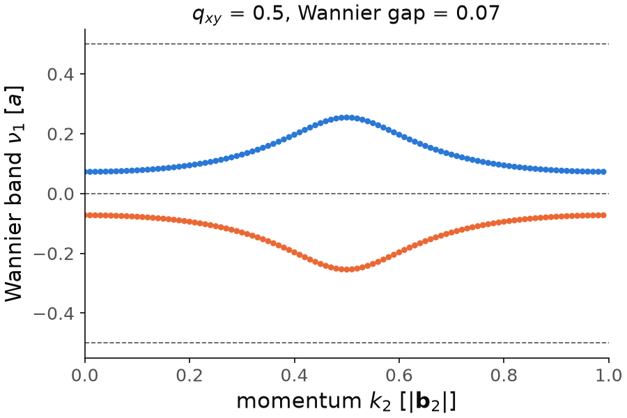
The figure shows the Wannier bands \(\nu_1(k_2)\) of the snippet, the hybrid Wannier centers along \(\vec a_1\) from topology.z2_wannier_centers(h,full=True). There are two, one per occupied band. They are mirror images of each other, and they form the two sectors: blue for \(\nu_1>0\) and orange for \(\nu_1<0\). They come closest to \(0\) at \(k_2=0\), at \(\pm0.073\), which is the value of topology.wannier_gap(h), and they reach \(\pm0.25\) at \(k_2=1/2\). They never touch \(0\) or \(1/2\), so the two sectors are well defined. The value of \(q_{xy}\) is not visible in this picture: it comes from the nested Wilson loop over each sector, which gives the four polarizations \(1/2\).

Code of this figure (documentation/figures/topology_quadrupole.py)

import numpy as np
import style
from pyqula import specialhamiltonian
from pyqula import topology
h = specialhamiltonian.square_2OTI(delta=0.3) # quadrupole insulator, four sites per cell with pi flux
q = h.get_quadrupole_moment() # quadrupole moment from the nested Wilson loops
p = h.get_wannier_sector_polarization(loop=0,sector="+") # polarization along a2 of one Wannier sector
w = topology.z2_wannier_centers(h,full=True) # Wannier bands nu_1(k_2), from the Wilson loop along b1
gap = topology.wannier_gap(h) # distance of the Wannier bands to 0 and 1/2

def draw(ax, c):
    for nu in np.array(w[1:])/(2*np.pi): # one Wannier band per occupied band
        ax.scatter(w[0], nu, s=10, color=np.where(nu>0, c.blue, c.orange)) # the two sectors
    for y in [-0.5,0,0.5]: ax.axhline(y, color=c.ink2, lw=0.8, ls="--")
    ax.set_ylim(-0.55, 0.55)
    ax.set_xlim(0, 1)
    ax.set_xlabel(r"momentum $k_2$ [$|\mathbf{b}_2|$]")
    ax.set_ylabel(r"Wannier band $\nu_1$ [$a$]")
    ax.set_title(f"$q_{{xy}}$ = {q:.1f}, Wannier gap = {gap:.2f}")

style.save(draw, "topology_quadrupole")

• nk: k-points per direction, 40 by default.
• gauge="atomic": put each orbital at its position in the cell. By default every orbital is at the origin of its cell, which is the convention that defines the quadrupole moment. With "atomic" the sector polarizations are positions in the unit cell.

See examples/2d/quadrupole/main.py for the invariant across the transition, examples/0d/cornermodes/main.py for the corner modes of the flake, and jupyter-notebooks/functionalities/topological_characterization/09_quadrupole_moment.ipynb.

Strong and weak Z2 indices in three dimensions

In three dimensions, h.get_topological_invariant() returns four \(Z_2\) indices. Take a plane of the Brillouin zone at a fixed momentum \(k_i\) along one reciprocal lattice vector. At \(k_i=0\) and at \(k_i=1/2\), time reversal maps the plane to itself, so each of these six planes is a two-dimensional time-reversal symmetric insulator, with its own \(Z_2\) invariant. Four combinations of them are independent, written \(\nu_0;(\nu_1\nu_2\nu_3)\):

• the weak index \(\nu_i\) is the invariant of the plane \(k_i=1/2\);
• the strong index \(\nu_0\) is the product of the invariants of the planes \(k_i=0\) and \(k_i=1/2\), which is the same for the three directions.

You can think of a weak topological insulator, \(\nu_0=0\) with some \(\nu_i=1\), as quantum spin Hall layers stacked along \(\nu_1\vec b_1+\nu_2\vec b_2+\nu_3\vec b_3\). It has Dirac cones only on the surfaces that cut the layers. A strong topological insulator, \(\nu_0=1\), has an odd number of Dirac cones on every surface, which is what ARPES sees.

We take the Fu-Kane-Mele model: the diamond lattice with spin-orbit coupling between second neighbors. The gap opens when one of the four first-neighbor bonds is different from the other three.

from pyqula import geometry
g = geometry.diamond_lattice_minimal() # diamond lattice, two sites per cell
h = g.get_hamiltonian() # first-neighbor hopping
h.add_kane_mele(0.05) # spin-orbit coupling between second neighbors
h.intra = 1.3*h.intra # make the bond inside the unit cell stronger
z2 = h.get_topological_invariant() # strong and weak Z2 indices

The result is (1, (1, 1, 1)), a strong topological insulator. With this bond weaker than the other three, h.intra = 0.7*h.intra, it is (0, (1, 1, 1)), a weak topological insulator of layers stacked along the bond. When the bond dominates, h.intra = 3.1*h.intra, it is (0, (0, 0, 0)), a band insulator of decoupled dimers.

Note that here the indices are 0 or 1, not the \(\pm 1\) of the two-dimensional invariant, because the weak ones are the components of a vector. They are given in the reciprocal lattice vectors of the geometry, so the weak vector depends on the choice of unit cell, but \(\nu_0\) does not. Each plane needs one two-dimensional invariant, with nk and nt as there, 60 by default. The call raises an error if the strong index is different for the three directions, which means that the flow of some plane was not resolved, or that the gap closes.

When time reversal is broken, the same call returns the Chern vector \((C_1,C_2,C_3)\): the Chern numbers of the planes at fixed \(k_1\), \(k_2\) and \(k_3\). For Chern insulator layers stacked along \(\vec a_3\) it is \((0,0,C)\), with \(C\) the Chern number of one layer, the Hall conductance of each layer in units of \(e^2/h\). Both are also available as topology.z2_invariant_3d(h) and topology.chern_vector(h). See examples/3d/z2_diamond/main.py for the three phases of the diamond model, and jupyter-notebooks/functionalities/topological_characterization/10_z2_three_dimensions.ipynb.

Winding number of a chiral chain

In one dimension h.get_topological_invariant() returns the Berry (Zak) phase. It is \(0\) or \(\pi\), so it only tells whether the number of zero modes at each end is even or odd. To count them we use h.get_winding_number().

The simplest case is the Su-Schrieffer-Heeger chain: two sites per cell, an intracell hopping \(t_1\) and an intercell hopping \(t_2\). The Hamiltonian only connects the two sublattices, so it anticommutes with the sublattice operator \(S\). This is called a chiral symmetry. In the eigenbasis of \(S\), the Bloch Hamiltonian is off-diagonal, with a block \(q(k)\) between the two sublattices. The winding number is

\[ W = \frac{1}{2\pi i}\oint dk\, \partial_k \log\det q(k) , \]

the number of times the phase of \(\det q(k)\) turns around when \(k\) crosses the Brillouin zone. It is the number of zero modes at each end of an open chain, all on one sublattice. STM sees them as a zero-bias peak at the end.

from pyqula import geometry
g = geometry.bichain() # two-site chain with a sublattice
def fun(r1,r2): # intracell hopping 0.5, intercell hopping 1
    dr = r1-r2
    if abs(dr.dot(dr)-1.)>1e-4: return 0. # first neighbors only
    return 0.5 if abs((r1[0]+r2[0])/2.)<1e-4 else 1.0 # the intracell bond is centered at x=0
h = g.get_hamiltonian(fun=fun,has_spin=False) # SSH chain
W = h.get_winding_number() # winding number, with the sublattice operator

The result is \(W=-1\), one zero mode at each end. It becomes \(0\) when the intracell hopping is the stronger one. The sign depends on which sublattice \(S\) counts as positive.

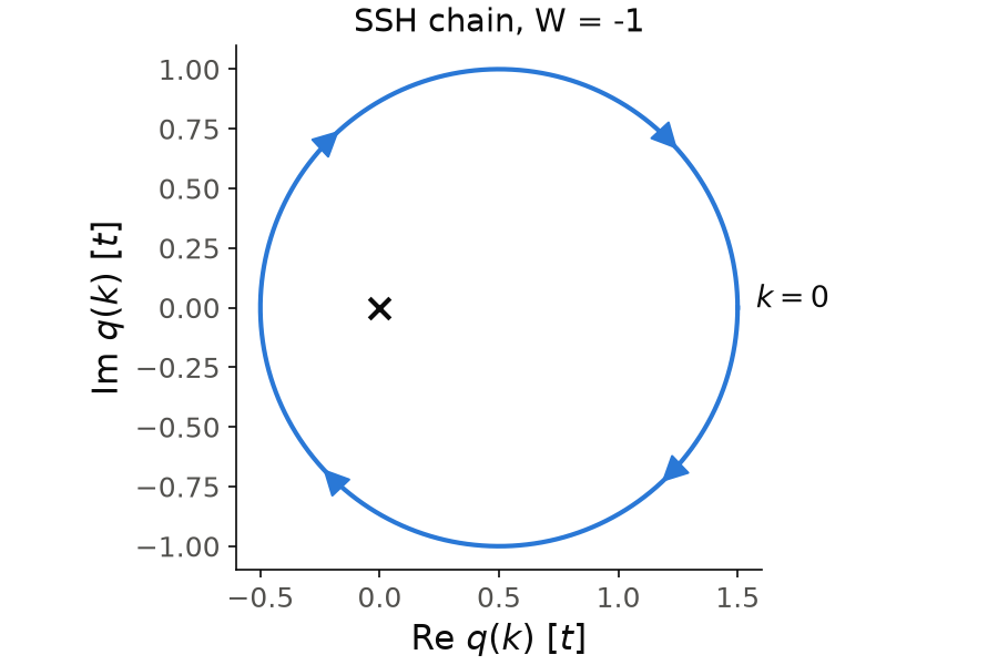
The figure shows \(q(k)\) of the snippet in the complex plane, as \(k\) crosses the Brillouin zone once. Each sublattice has one site, so \(q(k)\) is a single number, and here it is \(q(k)=0.5+e^{-ik}\), with \(k\) in units of the inverse lattice constant. This is a circle: its center is the intracell hopping \(0.5\), and its radius is the intercell hopping \(1\). So the circle goes around zero, the black cross, once and clockwise, and this is \(W=-1\). With the intracell hopping larger than the intercell one, the circle does not contain zero, and \(W=0\).

Code of this figure (documentation/figures/topology_winding.py)

import numpy as np
import style
from pyqula import geometry
g = geometry.bichain() # two-site chain with a sublattice
def fun(r1,r2): # intracell hopping 0.5, intercell hopping 1
    dr = r1-r2
    if abs(dr.dot(dr)-1.)>1e-4: return 0. # first neighbors only
    return 0.5 if abs((r1[0]+r2[0])/2.)<1e-4 else 1.0 # the intracell bond is centered at x=0
h = g.get_hamiltonian(fun=fun,has_spin=False) # SSH chain
W = h.get_winding_number() # winding number, with the sublattice operator
hk = h.get_hk_gen() # Bloch Hamiltonian H(k)
ks = np.linspace(0.,1.,200) # momenta across the Brillouin zone
q = np.array([hk([k,0.,0.])[0,1] for k in ks]) # off-diagonal block q(k), a number here

def draw(ax, c):
    ax.plot(q.real, q.imag, color=c.blue)
    for i in [25,75,125,175]: # arrows in the direction of growing k
        ax.annotate("", xy=(q[i+1].real,q[i+1].imag), xytext=(q[i].real,q[i].imag),
                    arrowprops=dict(arrowstyle="-|>", color=c.blue, mutation_scale=25))
    ax.annotate("$k=0$", (q[0].real,q[0].imag), xytext=(8,0), textcoords="offset points")
    ax.scatter([0], [0], marker="x", s=80, color=c.ink)
    ax.set_aspect("equal")
    ax.set_xlabel(r"Re $q(k)$ [$t$]")
    ax.set_ylabel(r"Im $q(k)$ [$t$]")
    ax.set_title(f"SSH chain, W = {W}")

style.save(draw, "topology_winding")

For a normal Hamiltonian the default chiral operator is the sublattice operator. For a Nambu Hamiltonian it is \(\sigma_y\tau_y\) on every site, the chiral symmetry of a BdG Hamiltonian that is real in real space. So the same call counts the Majorana zero modes of a Kitaev chain:

from pyqula import geometry
h = geometry.chain().get_hamiltonian() # spinful chain
h.add_onsite(20.) # shift both spin bands up
h.add_zeeman([0.,0.,20.]) # and bring one of them back to the Fermi energy
h.add_pairing(mode="pwave",delta=0.3,d=[1.,0.,0.]) # p-wave pairing: a Kitaev chain
W = h.get_winding_number() # sigma_y tau_y is the chiral operator by default

This gives \(W=1\) when the chemical potential is inside the band, and \(0\) outside. The difference with the Zak phase appears for two such chains coupled by a weak rung hopping: there are two Majorana zero modes at each end, \(W=2\), while the Zak phase gives \(0\), the same as a trivial chain.

• chiral: another chiral operator, as a name, a matrix or an Operator. The call raises an error if it does not anticommute with the Hamiltonian, or if the gap closes.

See examples/1d/winding_kitaev_ladder/main.py for the single chain and the ladder across the band, and jupyter-notebooks/functionalities/topological_characterization/11_one_dimensional_invariants.ipynb.

Z2 invariant of a helical superconducting wire

A wire with time-reversal symmetry, a class DIII superconductor, has a Kramers pair of Majorana zero modes at each end. This is a zero-bias peak that a magnetic field splits. The two invariants above do not see it: the Zak phase adds the two Kramers partners and is always trivial, and the winding with \(\sigma_y\tau_y\) counts them with opposite signs and gives \(0\). For a time-reversal symmetric Nambu chain, h.get_topological_invariant() returns instead the \(Z_2\) invariant, the Kramers polarization

\[ \nu = \det U \, \frac{\mathrm{Pf}\,\theta(0)}{\mathrm{Pf}\,\theta(\pi)} , \]

where \(U\) is the product of the overlaps of the negative-energy states from \(k=0\) to \(k=\pi\), and \(\theta\) is the time-reversal operator restricted to these states at the two time-reversal invariant momenta. So \(\nu\) compares how the Kramers partners are paired at the two ends of half of the Brillouin zone, and it is \(-1\) when they switch.

We take a helical p-wave wire, where the two spins pair with opposite chirality, with Rashba spin-orbit coupling so that spin is not conserved, and with a competing s-wave pairing:

from pyqula import geometry
h = geometry.chain().get_hamiltonian() # spinful chain
h.add_onsite(0.5) # shift the band, keeping the Fermi energy inside it
h.add_rashba(0.2) # Rashba spin-orbit coupling, so that spin is not conserved
h.add_pairing(mode="pwave",delta=0.5j,d=[1.,0.,0.]) # helical p-wave pairing
h.add_swave(0.2) # a competing s-wave pairing
nu = h.get_topological_invariant() # Z2 invariant of the wire

The result is \(-1\), a topological wire. When the s-wave pairing is larger than the p-wave one, h.add_swave(1.3), it is \(+1\), and the gap closes in between, near \(0.9\). When spin is conserved, without the Rashba coupling, \(\nu\) is the Zak parity of one spin block, a Kitaev chain.

• nk: number of k-points from \(0\) to \(\pi\), 200 by default. A value of \(\nu\) far from \(\pm 1\) raises an error, which asks for a larger nk.

It is also available as topology.z2_invariant_1d(h). See examples/1d/z2_helical_wire/main.py for the invariant as the s-wave pairing grows, and the 11_one_dimensional_invariants.ipynb notebook above.