Lattice gas models

A lattice gas describes classical particles that either occupy a site or not: adsorbates on a surface, vacancies in a crystal, or any classical order parameter with two values. We treat it with latticegas.LatticeGas.

The energy and the Monte Carlo sampling

The occupations are \(n_i\in\{0,1\}\), and the energy is

\[ E = \sum_{i\neq j} J_{ij}\, n_i n_j + \sum_i \mu_i n_i , \]

where \(J_{ij}\) is the interaction between two occupied sites and \(\mu_i\) is a chemical potential on each site. A positive \(J_{ij}\) is a repulsion. The sum runs over \(i\) and \(j\) separately, so each bond is counted twice. As for the classical spin models, the lattice and the neighbor shells come from a Geometry, and nothing else from the quantum Hamiltonian.

The configurations are sampled with Monte Carlo and the Metropolis rule. A move, the exchange of the occupations of two sites, changes the energy by \(\Delta E\), and it is accepted with probability \(\min\left(1, e^{-\Delta E/T}\right)\), with the temperature \(T\) in the same units as \(J\) (\(k_B=1\)). These exchange moves keep the number of particles fixed, so the filling, the fraction of occupied sites, does not change.

Ordering of repulsive particles

We take a triangular lattice with one third of the sites occupied, and a repulsion to first, second and third neighbors, so a pair of particles at the distance of first, second or third neighbors costs an energy \(J=1\):

from pyqula import geometry
from pyqula import supercell
from pyqula import latticegas

g = geometry.triangular_lattice()
g = supercell.turn_orthorhombic(g)
g = g.get_supercell(10) # periodic, so no site sits at an edge

lg = latticegas.LatticeGas(g,filling=1./3.) # 1/3 of the sites randomly occupied
lg.add_interaction(Jij=[1.,1.,1.]) # first, second and third neighbor repulsion
es = lg.optimize_energy(temp=0.5,ntries=1e4) # Metropolis run at fixed temperature

lg.den is the occupation of each site, 0 or 1, and es is the energy along the Monte Carlo run. The energy goes down and then becomes flat once the particles have found their arrangement. The supercell is periodic, so every site has the same neighbors as in the bulk. With g.dimensionality = 0 before building the model, the bonds across the border are cut instead, and we get a finite flake, where the sites at the edge have fewer neighbors and the order near the edge is different.

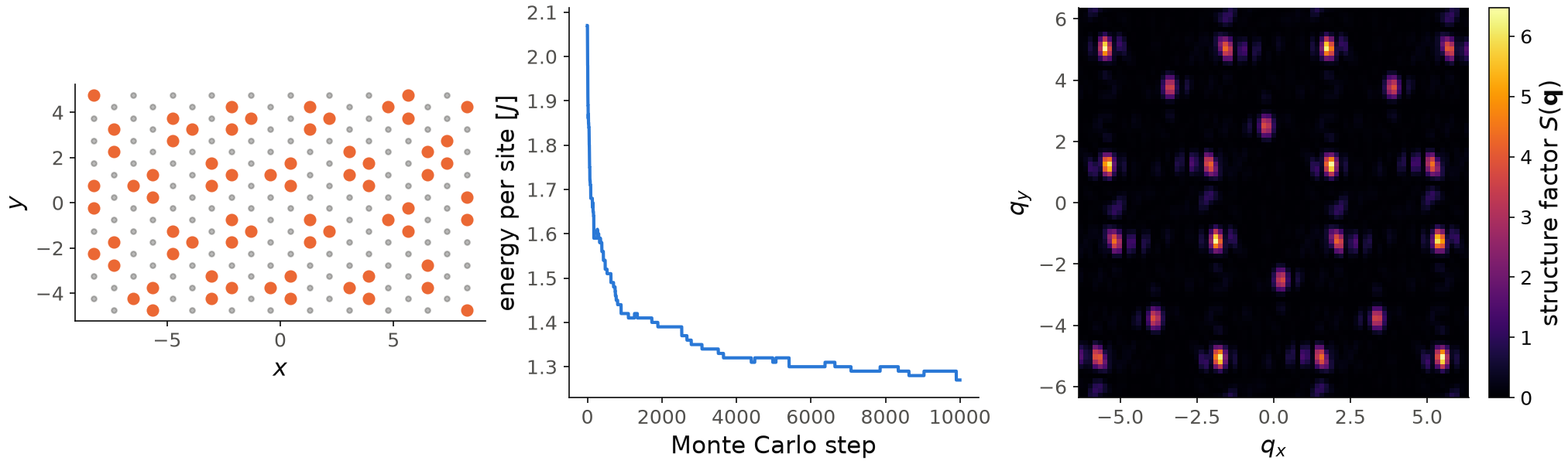
For the figure we also compute lg.get_structure_factor(nq=81), explained in the next paragraph. The energy per site (middle) goes down from 2.07 for the random start to 1.27, and after about 4000 moves it only decreases slowly. At one third filling the particles cannot avoid all the three shells of neighbors. In the run of the figure each occupied site (left, orange) has on average 2.0 occupied first neighbors, 1.1 second and 0.66 third neighbors, so the particles form chains, and the energy per site is \((2.0+1.1+0.66)/3\approx1.27\). The structure factor (right) is zero at \(\mathbf q=0\), and it has sharp peaks at finite \(\mathbf q\), so the occupations are ordered. The script fixes the random seed. With another seed the positions of the peaks and the final energy change a little: one run of \(10^4\) moves is 50 moves per site, and it can stop with domains of different orientations.

Code of this figure (documentation/figures/latticegas_order.py)

import numpy as np
import style
from pyqula import geometry
from pyqula import supercell
from pyqula import latticegas
np.random.seed(1) # fixed seed, so that every run gives the same figure

g = geometry.triangular_lattice()
g = supercell.turn_orthorhombic(g)
g = g.get_supercell(10) # periodic, so no site sits at an edge

lg = latticegas.LatticeGas(g,filling=1./3.) # 1/3 of the sites randomly occupied
lg.add_interaction(Jij=[1.,1.,1.]) # first, second and third neighbor repulsion
es = lg.optimize_energy(temp=0.5,ntries=1e4) # simulated annealing
(q,sq) = lg.get_structure_factor(nq=81) # structure factor on a grid of q

def draw(ax, c):
    occ = lg.den > 0.5 # occupied sites
    ax[0].scatter(g.r[:,0], g.r[:,1], s=10, color=c.ink2, alpha=0.4)
    ax[0].scatter(g.r[occ,0], g.r[occ,1], s=45, color=c.orange)
    ax[0].set_aspect("equal")
    ax[0].set_xlabel("$x$") ; ax[0].set_ylabel("$y$")
    ax[1].plot(es/len(g.r), color=c.blue)
    ax[1].set_xlabel("Monte Carlo step")
    ax[1].set_ylabel("energy per site [$J$]")
    n = int(np.sqrt(len(sq)))
    im = ax[2].pcolormesh(q[:,0].reshape(n,n), q[:,1].reshape(n,n),
                          sq.reshape(n,n), cmap=c.cmap, shading="auto")
    style.colorbar(im, ax[2], r"structure factor $S(\mathbf{q})$")
    ax[2].set_aspect("equal")
    ax[2].set_xlabel("$q_x$") ; ax[2].set_ylabel("$q_y$")

style.save(draw, "latticegas_order", npanels=3)

To find which order the particles form, look at the density-density correlator in real space, get_correlator(), and in reciprocal space, get_structure_factor(). The structure factor has peaks at the ordering wavevector of the ordered state, for example a stripe order or a honeycomb arrangement of vacancies. This is the quantity that diffraction measures.

Keywords and other methods

• temp: temperature \(T\); higher values accept more moves that increase the energy.
• ntries: number of attempted moves.
• anneal(): runs optimize_energy() with a decreasing temperature and keeps the best configuration, so the system does not stay in a local minimum.
• optimize_energy_multistart(): keeps the best of several independent runs.
• optimize_grand_canonical(): flips single occupations at chemical potential lg.mu, so the filling changes; use it to scan the filling as a function of the chemical potential.
• get_specific_heat(), get_susceptibility(): thermodynamic quantities from the fluctuations along a run at fixed temperature.
• get_local_energy(), get_local_mu(): the energy of each site, and the cost \(\mu_i+\sum_k J_{ik}n_k\) of occupying it, in the current configuration.
• add_tensor(): couplings that are not given by neighbor shells.
• write(), read(): save a configuration to a file and read it back.

See examples/latticegas/ for runnable scripts of the annealing, the map of the local energy, the correlators, and the scan of the filling against the chemical potential, and jupyter-notebooks/functionalities/classical_spin_models_monte_carlo/03_lattice_gas_monte_carlo.ipynb and 05_correlators_thermodynamics.ipynb in the same folder for executed notebooks.