Non-Hermitian Hamiltonians

An open system exchanges particles or energy with an environment. Such a system is often described by an effective Hamiltonian that is not Hermitian. Gain and loss appear as imaginary onsite energies, \(\epsilon_n \to \epsilon_n + i\gamma_n\), with \(\gamma_n>0\) for gain and \(\gamma_n<0\) for loss. A non-reciprocal hopping, \(t_{ij}\neq t_{ji}^*\), appears as a hopping matrix that is not Hermitian. The eigenvalues \(E_n\) are then complex. The real part is an energy, and the imaginary part is a rate: a state evolves as \(e^{-iE_nt}\), so it grows if \(\mathrm{Im}\,E_n>0\) and decays if \(\mathrm{Im}\,E_n<0\). The eigenvectors are not orthogonal anymore. This is the physics of photonic and acoustic lattices with gain and loss, of the non-Hermitian skin effect, and of \(\mathcal{PT}\)-symmetric models, and also of quasiparticles with a finite lifetime.

A non-Hermitian Hamiltonian is generated with non_hermitian=True in g.get_hamiltonian(). The model is then built as usual; for example, gain and loss are added with h.add_onsite() and a complex function. Let us take a chain of twenty sites with a purely imaginary modulation of the onsite energy,

\[ H = -\sum_n \left(c^\dagger_n c_{n+1} + h.c.\right) + i\,0.6 \sum_n \cos\!\left(\frac{2\pi x_n}{20}\right) c^\dagger_n c_n , \]

with gain where the cosine is positive and loss where it is negative:

import numpy as np
from pyqula import geometry

n = 20
g = geometry.chain().get_supercell(n)
h = g.get_hamiltonian(has_spin=False,non_hermitian=True,tij=[-1.])
# a purely imaginary Aubry-Andre modulation, with no Hermitian part at
# all: gain where the cosine is positive, loss where it is negative
h.add_onsite(lambda r: 0.6j*np.cos(2.*np.pi*r[0]/n))

(ks,es) = h.get_bands(kpath=[[0.,0.,0.]],write=False)
print("eigenvalues are complex:",es.dtype)
print("largest gain rate Im(E):",np.round(np.max(es.imag),4))

The eigenvalues are complex: twenty of them, one per site. The real parts are inside the band of the chain, between \(-2\) and \(2\). The imaginary parts are between \(-0.48\) and \(+0.48\), smaller than the \(0.6\) of the modulation, because the hopping mixes sites with gain and sites with loss. To plot them you have to choose: es.real for the energy, es.imag for the gain or decay rate, or both in the complex plane.

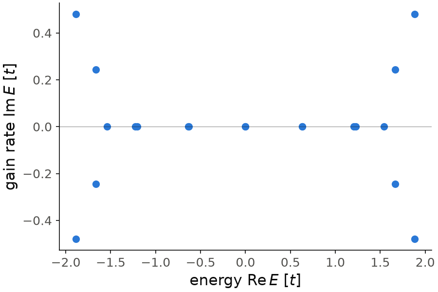
Each dot is one eigenvalue, with the energy on the horizontal axis and the gain rate on the vertical one. Twelve of the twenty eigenvalues are real, between \(-1.54\) and \(1.54\): these states are spread equally over the gain and the loss, so they neither grow nor decay. The other eight are close to the band edges, at \(|\mathrm{Re}\,E|\) between \(1.67\) and \(1.88\), and come in pairs \(E\) and \(E^*\), with rates \(\pm0.25\) and \(\pm0.48\). The spectrum is also symmetric under \(E\to-E\).

Code of this figure (documentation/figures/nonhermitian_spectrum.py)

import numpy as np
import style
from pyqula import geometry

n = 20
g = geometry.chain().get_supercell(n)
h = g.get_hamiltonian(has_spin=False,non_hermitian=True,tij=[-1.])
# a purely imaginary Aubry-Andre modulation, with no Hermitian part at
# all: gain where the cosine is positive, loss where it is negative
h.add_onsite(lambda r: 0.6j*np.cos(2.*np.pi*r[0]/n))

(ks,es) = h.get_bands(kpath=[[0.,0.,0.]],write=False)
print("eigenvalues are complex:",es.dtype)
print("largest gain rate Im(E):",np.round(np.max(es.imag),4))

def draw(ax, c):
    ax.axhline(0, color=c.ink, lw=0.6, alpha=0.4)
    ax.scatter(es.real, es.imag, s=40, color=c.blue)
    ax.set_xlabel(r"energy Re$\,E$ [$t$]")
    ax.set_ylabel(r"gain rate Im$\,E$ [$t$]")

style.save(draw, "nonhermitian_spectrum")

Choosing which part is the energy: eigmode

The argument eigmode says which part of the complex eigenvalue is used as the energy. It can be

• "complex" (default): the whole complex eigenvalue.
• "real": the real part, the energy.
• "imag": the imaginary part, the gain or decay rate.

In h.get_bands() it decides what the returned energies contain. With "complex" the file BANDS.OUT has one more column, with the columns k, \(\mathrm{Re}\,E\), \(\mathrm{Im}\,E\), and then one column per operator.

In h.get_ldos() it decides on which axis the energy e is. With eigmode="imag" the states are selected by their gain rate and not by their energy. In this way we can ask where the most amplified state of the chain above is located:

import numpy as np
from pyqula import geometry
n = 20
g = geometry.chain().get_supercell(n)
h = g.get_hamiltonian(has_spin=False,non_hermitian=True,tij=[-1.])
h.add_onsite(lambda r: 0.6j*np.cos(2.*np.pi*r[0]/n))
(ks,es) = h.get_bands(kpath=[[0.,0.,0.]],write=False)

imax = np.argmax(es.imag) # the most amplified state
(x,y,d) = h.get_ldos(e=es[imax].imag,delta=1e-2,eigmode="imag",nrep=1)
print("it lives at x =",x[np.argmax(d)])

The answer is \(x=-0.5\), the site where the gain is largest. As expected, the most amplified state lives where the imaginary onsite energy is largest.

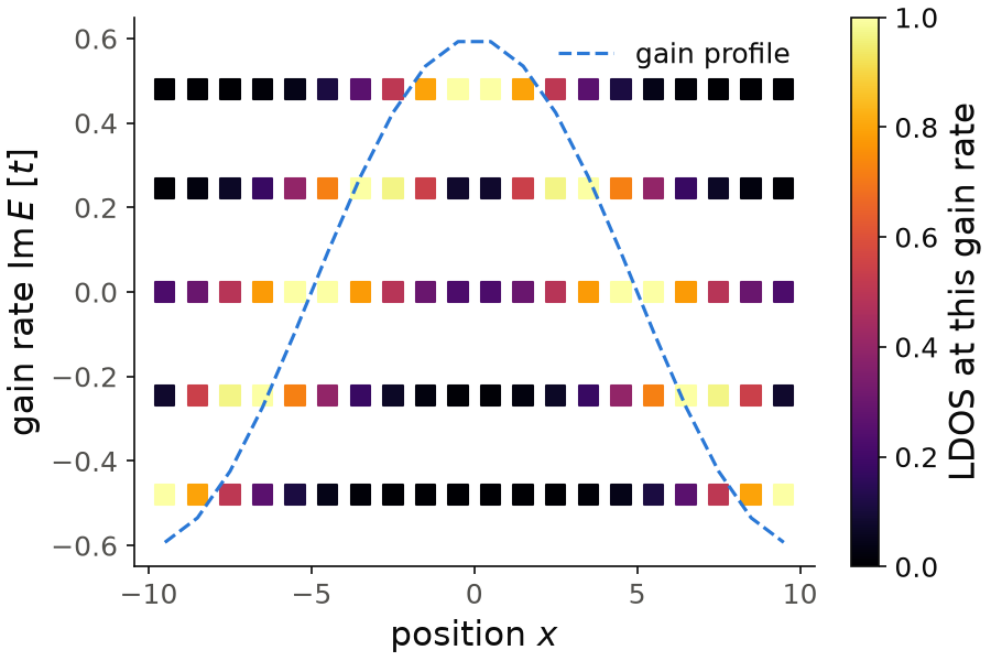
Each row is the map d at one of the five gain rates of the spectrum, computed in the same way as in the snippet, and normalized to its largest value. The dashed line is the gain \(0.6\cos(2\pi x/20)\) of each site. The states with the largest gain, \(\mathrm{Im}\,E=0.48\), live around \(x=0\), where the gain is largest, and the states with the largest loss, \(\mathrm{Im}\,E=-0.48\), live around \(x=\pm10\), where the loss is largest. The real states, \(\mathrm{Im}\,E=0\), have their weight around \(x=\pm5\), where the onsite energy is zero.

Code of this figure (documentation/figures/nonhermitian_eigmode.py)

import numpy as np
import style
from pyqula import geometry
n = 20
g = geometry.chain().get_supercell(n)
h = g.get_hamiltonian(has_spin=False,non_hermitian=True,tij=[-1.])
h.add_onsite(lambda r: 0.6j*np.cos(2.*np.pi*r[0]/n))
(ks,es) = h.get_bands(kpath=[[0.,0.,0.]],write=False)

imax = np.argmax(es.imag) # the most amplified state
(x,y,d) = h.get_ldos(e=es[imax].imag,delta=1e-2,eigmode="imag",nrep=1)
print("it lives at x =",x[np.argmax(d)])

rates = np.unique(es.imag.round(4)) # the different gain rates
ldos = [h.get_ldos(e=w,delta=1e-2,eigmode="imag",nrep=1)[2] for w in rates]
ldos = [d/d.max() for d in ldos] # each row normalized to its largest value

def draw(ax, c):
    for (w,d) in zip(rates,ldos):
        sc = ax.scatter(x, w+0*x, c=d, s=70, marker="s", cmap=c.cmap, vmin=0, vmax=1)
    style.colorbar(sc, ax, "LDOS at this gain rate")
    ax.plot(x, 0.6*np.cos(2*np.pi*x/n), "--", color=c.blue, lw=1.5, label="gain profile")
    ax.set_xlabel("position $x$")
    ax.set_ylabel(r"gain rate Im$\,E$ [$t$]")
    ax.set_ylim(-0.65, 0.65)
    ax.legend(loc="upper right")

style.save(draw, "nonhermitian_eigmode")

h.get_dos() always broadens the real part when eigmode is "complex" or "real", so both give the same density of states. With "imag" it gives the distribution of the gain and decay rates.

The two spectral functions of a non-Hermitian Hamiltonian

We now see that a non-Hermitian Hamiltonian has two different momentum-resolved spectral functions, and how to compute each one with h.get_kdos_bands(). A non-Hermitian Hamiltonian has right eigenvectors \(|R_n\rangle\) and left eigenvectors \(\langle L_n|\),

\[ H|R_n\rangle = E_n|R_n\rangle, \qquad \langle L_n|H = E_n\langle L_n| , \]

and they are different. The weight of an operator \(O\) in a state can be defined with the right eigenvector alone, or with both:

\[ O^{R}_n = \frac{\langle R_n|O|R_n\rangle}{\langle R_n|R_n\rangle}, \qquad O^{LR}_n = \frac{\langle L_n|O|R_n\rangle}{\langle L_n|R_n\rangle} . \]

The first one is the default of h.get_kdos_bands(). Each state gives a Lorentzian of width delta at \(\mathrm{Re}\,E_n\), with a positive weight for a positive operator. This is the usual picture of a band structure.

The second one is what the Green's function gives,

\[ A(\mathbf k,\omega) = -\frac{1}{\pi}\,\mathrm{Im}\,\mathrm{Tr}\left[O\,(\omega+i\delta-H_{\mathbf k})^{-1}\right] = -\frac{1}{\pi}\,\mathrm{Im}\sum_n \frac{O^{LR}_n}{\omega+i\delta-E_n} . \]

Here a state with \(\mathrm{Im}\,E_n<0\) is broadened by its own decay rate, its finite lifetime. This is how an effective non-Hermitian Hamiltonian describes quasiparticles that decay, and it is the spectral function that ARPES measures for such quasiparticles. It is computed with biorthogonal=True:

import numpy as np
from pyqula import geometry
g = geometry.chain().get_supercell(4,store_primal=True) # supercell of a chain
h = g.get_hamiltonian(has_spin=False,non_hermitian=True) # non-Hermitian Hamiltonian
h.add_onsite(lambda r: -0.3j*(1.+np.cos(np.pi*r[0]/2.))) # modulated loss
kpath = g.get_unfolded_kpath(nk=400) # primitive k-path, in supercell coordinates
(k,e,d) = h.get_kdos_bands(operator="unfold",kpath=kpath,
        biorthogonal=True) # unfolded Green's-function spectral function

Compared with the default, each unfolded band is broader and lower, because of the loss of its states. The two spectral functions are the same when the spectrum is real. Otherwise they differ in two ways. The Green's function one includes the lifetime of each state. And its weight can be negative for a state with gain, \(\mathrm{Im}\,E_n>0\), whose pole is on the wrong side of the real axis. Close to an exceptional point, where two eigenvectors become the same, the biorthogonal weights of the two states become large and cancel each other, and only their sum has a meaning.

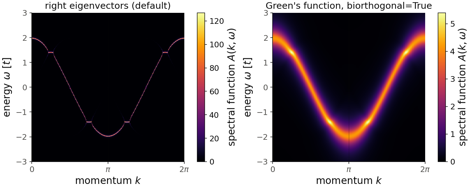
For the figure we use a finer energy grid than the default, energies=np.linspace(-3.,3.,1201), so that the sharp peaks of the left panel are not lost between two energies. The 400 points of the k-path are needed for the same reason: with 100 points the band moves by more than \(\delta\) from one k-point to the next, and the left panel shows a dotted line. In both panels you see the cosine band of the chain, from \(2\) at \(k=0\) to \(-2\) at \(k=\pi\). All the states have the same decay rate here, \(\mathrm{Im}\,E_n=-0.3\), the average loss of the four sites. In the left panel the peaks have the width \(\delta=0.01\) and a height of up to \(127\), so the band is a thin line. In the right panel each peak has a full width of \(0.61\), which is \(2(0.3+\delta)\), and a height of about \(4.2\), so the lifetime of the states is visible. Around \(\omega=\pm1.4\) two folded bands of the supercell meet, and there the weight goes up to \(5.4\).

Code of this figure (documentation/figures/nonhermitian_kdos.py)

import numpy as np
import style
from pyqula import geometry
g = geometry.chain().get_supercell(4,store_primal=True) # supercell of a chain
h = g.get_hamiltonian(has_spin=False,non_hermitian=True) # non-Hermitian Hamiltonian
h.add_onsite(lambda r: -0.3j*(1.+np.cos(np.pi*r[0]/2.))) # modulated loss
kpath = g.get_unfolded_kpath(nk=400) # primitive k-path, in supercell coordinates
(k,e,d) = h.get_kdos_bands(operator="unfold",kpath=kpath,
        biorthogonal=True) # unfolded Green's-function spectral function
es = np.linspace(-3.,3.,1201) # a finer energy grid than the default, for the figure
(k,e,d) = h.get_kdos_bands(operator="unfold",kpath=kpath,energies=es,biorthogonal=True)
(k0,e0,d0) = h.get_kdos_bands(operator="unfold",kpath=kpath,energies=es) # the default one

nk, ne = len(kpath), len(es) # the arrays are flat, k-point by k-point
K = 2*np.pi*k.reshape(nk,ne)/k.max() # momentum of the primitive chain
E = e.reshape(nk,ne)

def draw(axs, c):
    for (ax,dd,title) in zip(axs, [d0,d], ["right eigenvectors (default)",
                                         "Green's function, biorthogonal=True"]):
        m = ax.pcolormesh(K, E, dd.reshape(nk,ne), cmap=c.cmap, vmin=0,
                          vmax=dd.max(), shading="nearest")
        style.colorbar(m, ax, r"spectral function $A(k,\omega)$")
        style.kpath(ax, K.ravel(), ["0", r"$\pi$", r"$2\pi$"])
        ax.set_xlabel("momentum $k$")
        ax.set_ylabel(r"energy $\omega$ [$t$]")
        ax.set_title(title)

style.save(draw, "nonhermitian_kdos", npanels=2)

The same choice exists in other functions:

• mode="green" in h.get_kdos_bands() computes the Green's function spectral function directly, so it needs biorthogonal=True for a non-Hermitian Hamiltonian.
• h.get_bands(operator=...,biorthogonal=True) returns the weights \(O^{LR}_n\) state by state. They are complex in general, and at each k-point they add up to the trace of the operator.
• h.get_dos(biorthogonal=True) sums the Green's function spectral function over the Brillouin zone.

What is and is not available

These quantities have a real non-Hermitian version: the band structure, the density of states, the local density of states, the Berry curvature and the density matrix. The occupied states are those with the lowest real part of the energy. Each of them enters with its right and left eigenvectors, normalized so that \(\langle L|R\rangle=1\), and the density matrix is

\[ \rho = \sum_{n\in{\rm occ}} |R_n\rangle\langle L_n| . \]

An expectation value is then \(\langle A\rangle = \mathrm{Tr}(\rho A) = \sum_{\rm occ} \langle L_n|A|R_n\rangle\), complex in general. h.get_density_matrix() gives this \(\rho\), and h.get_vev() and h.get_magnetization() give the real part of the expectation value. The self-consistent mean field also uses this \(\rho\), so the mean-field Hamiltonian is itself non-Hermitian.

A simple check is the open Hatano-Nelson chain, with hopping \(t_R\) to the right and \(t_L\) to the left. An imaginary gauge transformation turns it into a Hermitian chain with hopping \(\sqrt{t_Rt_L}\), without changing any density. So with a Hubbard \(U\) its self-consistent spectrum is the one of the Hermitian chain (see jupyter-notebooks/functionalities/interacting_mean_field_hamiltonians/08_hermitian_nonhermitian.ipynb).

This works with exact diagonalization, for a Hamiltonian without superconductivity. The kernel polynomial method, use_jax=True and integration="qtci" assume a real spectrum, and raise a NotImplementedError. In the same way, h.get_dos() accepts only mode="ED". h.get_ldos() only works with its default mode, so do not pass another one. Other quantities use the Hermitian formula on a non-Hermitian Hamiltonian, which may or may not have a meaning for a complex spectrum, so check before you use them.

Operators work as usual, also operator="unfold", so a supercell can be unfolded to the primitive Brillouin zone with a complex spectrum; see examples/1d/unfolding_non_hermitian/main.py. num_bands also works, and gives the few eigenvalues closest to central_energy.

See examples/1d/NH_ldos/main.py (the model above, state by state), examples/0d/non_hermitian_aah/main.py and examples/0d/non_hermitian_aah_dos/main.py (a non-Hermitian Aubry-André chain as a function of the phase of the modulation) for runnable scripts, and jupyter-notebooks/functionalities/single_particle_hamiltonians/09_non_hermitian_hamiltonians.ipynb for an executed notebook.