Ising models

The Ising model has a classical spin \(s_i\in\{-1,+1\}\) on each site. We treat it with latticeising.LatticeIsing, which works in the same way as the lattice gas.

The energy

The energy is

\[ E = -\sum_{i\neq j} J_{ij}\, s_i s_j - \sum_i b_i s_i , \]

where \(J_{ij}\) is the coupling between two spins and \(b_i\) is a magnetic field on each site. A positive \(J_{ij}\) is ferromagnetic, it favors parallel spins. Note that the sign convention is the opposite of the lattice gas, where the coupling has no minus sign and a positive \(J\) is a repulsion.

The sum runs over \(i\) and \(j\) separately, so each bond is counted twice, and the energy is two times the usual sum over bonds. As a result, all the energies and temperatures are two times larger than in the usual convention. For example, the ferromagnet on the square lattice orders at \(T_c = 2\times 2.269\,J \approx 4.54\,J\), not at \(2.269\,J\).

The spins are sampled with Monte Carlo and the Metropolis rule, as in the lattice gas: a move that changes the energy by \(\Delta E\) is accepted with probability \(\min\left(1,e^{-\Delta E/T}\right)\), with \(k_B=1\).

The ferromagnetic transition

The simplest case is a ferromagnet on the square lattice. The lattice is bipartite, so nothing frustrates the order:

from pyqula import geometry
from pyqula import latticeising

g = geometry.square_lattice() # bipartite, so ferromagnetic order is not frustrated
g = g.get_supercell(12) # periodic, so no site sits at an edge

li = latticeising.LatticeIsing(g,m=0.0) # random +-1 spins, zero net magnetization
li.add_interaction(Jij=[1.]) # first-neighbor ferromagnetic coupling
es,ms = li.anneal(temps=[3.,1.,0.3,0.1,0.03],ntries=1e4) # simulated annealing

li.s contains the spins, \(\pm1\), es the energy along the run, and ms the total magnetization \(\sum_i s_i\) along the run. In ms you see the phase transition. All the temperatures of the snippet are below \(T_c\approx4.54\,J\), so already in the first stage, at \(T=3\), the magnetization per site ms/li.nsites grows from zero to \(+1\) or \(-1\), all the spins parallel, and the sign is chosen at random. To see the disordered phase, where the magnetization fluctuates around zero, add a first stage above \(T_c\), as in the figure below. As in the lattice gas, the supercell is periodic, and g.dimensionality = 0 makes it a finite flake.

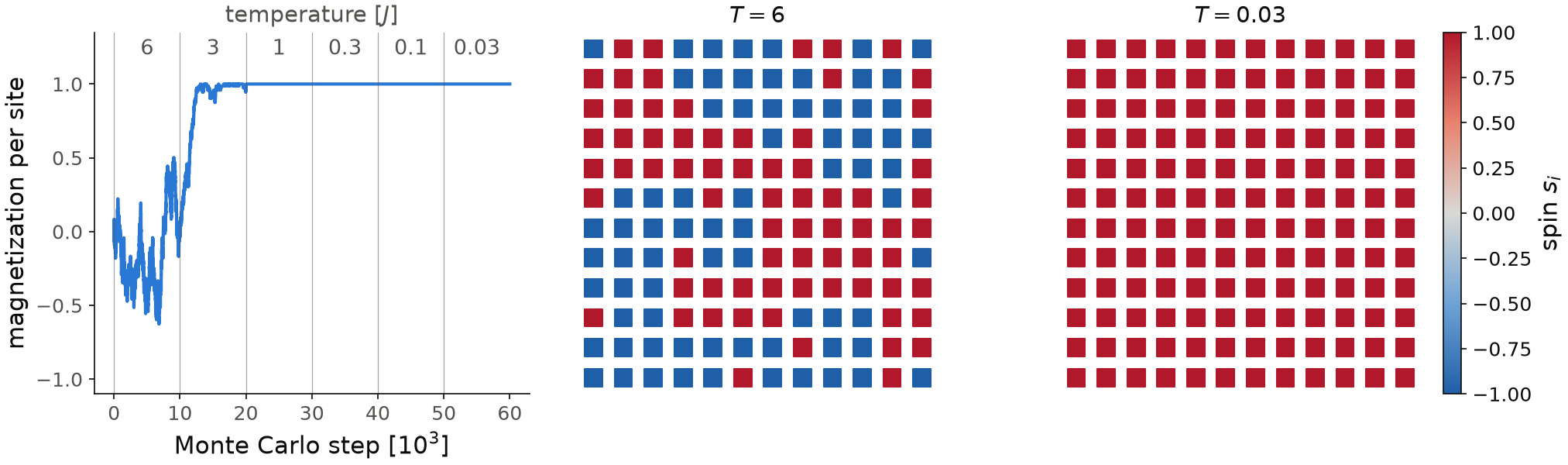
For the figure we add a first stage at \(T=6\), above \(T_c\), and we keep the spins at its end with checkpoint_at. At \(T=6\) the magnetization per site (left) fluctuates around zero, between \(-0.6\) and \(0.5\) on this small lattice, and the spins form domains of both signs (middle). At \(T=3\) it grows to \(+1\) after about 3000 steps, and it stays there at the lower temperatures. At the end all the spins are parallel (right), and the energy is \(-4J\) per site, two times the \(-2J\) of the usual sum over bonds.

Code of this figure (documentation/figures/ising_ferro.py)

import numpy as np
import style
from pyqula import geometry
from pyqula import latticeising
np.random.seed(1) # fixed seed, so that every run gives the same figure

g = geometry.square_lattice() # bipartite, so ferromagnetic order is not frustrated
g = g.get_supercell(12) # periodic, so no site sits at an edge

li = latticeising.LatticeIsing(g,m=0.0) # random +-1 spins, zero net magnetization
li.add_interaction(Jij=[1.]) # first-neighbor ferromagnetic coupling
temps = [6.,3.,1.,0.3,0.1,0.03] # the figure starts above Tc=4.54
es,ms = li.anneal(temps=temps,ntries=1e4,checkpoint_at=10000) # simulated annealing
s_hot = li.checkpoints[10000] # spins at the end of the stage at T=6

def spins(ax, s, title, c):
    sc = ax.scatter(g.r[:,0], g.r[:,1], c=s, s=120, marker="s",
                    cmap=c.diverging, vmin=-1, vmax=1)
    ax.set_aspect("equal") ; ax.set_axis_off()
    ax.set_title(title)
    return sc

def draw(ax, c):
    n = len(ms)//len(temps) # Monte Carlo steps per temperature
    ax[0].plot(np.arange(len(ms))/1e3, ms/li.nsites, color=c.blue)
    for i,T in enumerate(temps):
        ax[0].axvline(i*n/1e3, color=c.ink2, lw=0.6, alpha=0.5)
        ax[0].text((i+0.5)*n/1e3, 1.2, f"{T:g}", ha="center", color=c.ink2)
    ax[0].set_title("temperature [$J$]", color=c.ink2)
    ax[0].set_ylim(-1.1, 1.35)
    ax[0].set_xlabel("Monte Carlo step [$10^3$]")
    ax[0].set_ylabel(r"magnetization per site")
    spins(ax[1], s_hot, "$T=6$", c)
    sc = spins(ax[2], li.s, "$T=0.03$", c)
    style.colorbar(sc, ax[2], "spin $s_i$")

style.save(draw, "ising_ferro", npanels=3)

Keywords and other methods

• li.optimize_energy(): Metropolis with single spin flips; the magnetization is not conserved. Returns the energy and the total magnetization along the run, (es, ms), and ms can be given to latticegas.get_susceptibility().
• li.optimize_conserved(): Kawasaki dynamics, exchanges of two spins; the total magnetization is conserved, as the filling in the lattice gas.
• li.anneal(): optimize_energy() with a decreasing temperature, given by temps.
• optimize_energy_multistart(): keeps the best of several independent runs.
• get_local_energy(), get_local_field(): the energy and the effective field of each site in the current configuration.
• get_correlator(), get_structure_factor(): spin-spin correlator in real and reciprocal space; the peak gives the ordering wavevector, \(\Gamma\) for a ferromagnet and \(M\) for the checkerboard antiferromagnet.
• add_tensor(), regroup(), get_specific_heat(), get_susceptibility(): the same as in the lattice gas.

See examples/latticeising/ for runnable scripts of the annealing, a scan in temperature (magnetization and specific heat), and maps of the local energy and field of a frustrated antiferromagnet on the triangular lattice, and jupyter-notebooks/functionalities/classical_spin_models_monte_carlo/04_ising_monte_carlo.ipynb and 05_correlators_thermodynamics.ipynb in the same folder for executed notebooks.