Spin susceptibility, RPA and magnons

In Charge response and RKKY we computed the bare response of non-interacting electrons. Now we add the interactions, in the random phase approximation (RPA), and we find the collective modes of an interacting state: magnons in a magnet and plasmons in the charge channel. The interacting state is a mean-field Hamiltonian, obtained as in Mean-field Hubbard models.

Spin susceptibility in the RPA

When we perturb an interacting system, the perturbation moves some electrons, this changes the mean field that the other electrons feel, and this moves more electrons. Summing this series gives the RPA response,

\[ \chi_{\rm RPA}(q,\omega) = \chi_0(q,\omega)\,\left[1 - V(q)\,\chi_0(q,\omega)\right]^{-1}, \]

where \(\chi_0\) is the bare response matrix of the mean-field Hamiltonian, with one entry per site and per operator, and \(V(q)\) is the interaction vertex in the same channel. For the spin response the vertex is built from the Hubbard \(U\) stored on the mean-field Hamiltonian. In a magnetically ordered state, the RPA response has the magnons, which the bare response does not have. It is computed with

• h.get_spinchi_ladder(): the transverse response, between \(S^+\) and \(S^-\), where the magnons appear.
• h.get_spinchi_full(): the full tensor between \(S_x\), \(S_y\) and \(S_z\).

We converge an antiferromagnetic chain and compute its transverse response at a small momentum transfer:

from pyqula import geometry
import numpy as np
g = geometry.bichain() # two sites per cell, so Neel order fits in the cell
h = g.get_hamiltonian(has_spin=True)
seed = h.copy() ; seed.add_antiferromagnetism(0.5) # symmetry-breaking seed
hmf = h.get_mean_field_hamiltonian(U=3.0,filling=0.5,mf=seed,nk=100) # magnetic state
(es,chis) = hmf.get_spinchi_ladder(energies=np.linspace(0.,2.,400),q=[0.1,0.,0.],nk=40,delta=2e-2)

The imaginary part of chis has a sharp peak at the magnon energy at this \(q\). This is what inelastic neutron scattering measures in a magnet. Without spin-orbit coupling the peak goes to zero energy at \(q=0\): it is the Goldstone mode of the broken spin-rotation symmetry.

The keywords are

• q: the momentum transfer, in units of the reciprocal lattice vectors. Without q, the response is dressed at every \(q\) of the k-mesh and then averaged, which gives the local response, the one a probe on a single site sees.
• RPA: True (default) dresses the response with the interaction; False gives the bare response.
• energies, delta, nk: frequencies, broadening and k-mesh, as for h.get_chi().

Two related methods use the same response:

• h.get_qdos_iets() scans get_spinchi_full along a q-path, so it gives the dispersion of the spin excitations along high-symmetry directions.
• h.get_iets_ldos() computes the local response at one energy on every site, which is the map of the spin-flip signal that inelastic tunneling spectroscopy (IETS) measures with an STM. Together with h.get_ldos() it gives the elastic and inelastic STM maps.

The q-path labels "G","K","M" need a two-dimensional lattice. On the antiferromagnetic honeycomb lattice, the dispersion along the path is

g2 = geometry.honeycomb_lattice() # already two sublattices per cell
h2 = g2.get_hamiltonian(has_spin=True)
hmf2 = h2.get_mean_field_hamiltonian(U=3.0,filling=0.5,mf="antiferro")
qdisp = hmf2.get_qdos_iets(energies=np.linspace(0.,2.,250),qpath=["G","K","M"],nq=120,nk=60,delta=1e-2)

Before reading the spectrum, check that the mean-field state is really ordered, with hmf.get_vev("sz"). An RPA calculation on a non-magnetic state runs without problems, but it has no magnons. Two things decide whether the state is ordered. First, the unit cell must be able to hold the order: a geometry.chain() has one site per cell and cannot have Néel order, while bichain and honeycomb_lattice have two sublattices. Second, \(U\) must be larger than the critical value: on the honeycomb lattice at half filling \(U=2\) gives a moment of 0.002, so no order, and \(U=3\) gives 0.44. The cost of get_qdos_iets grows with nq, with the number of energies and with the number of k-points, \(n_k^2\) in two dimensions: the grid above takes about five minutes.

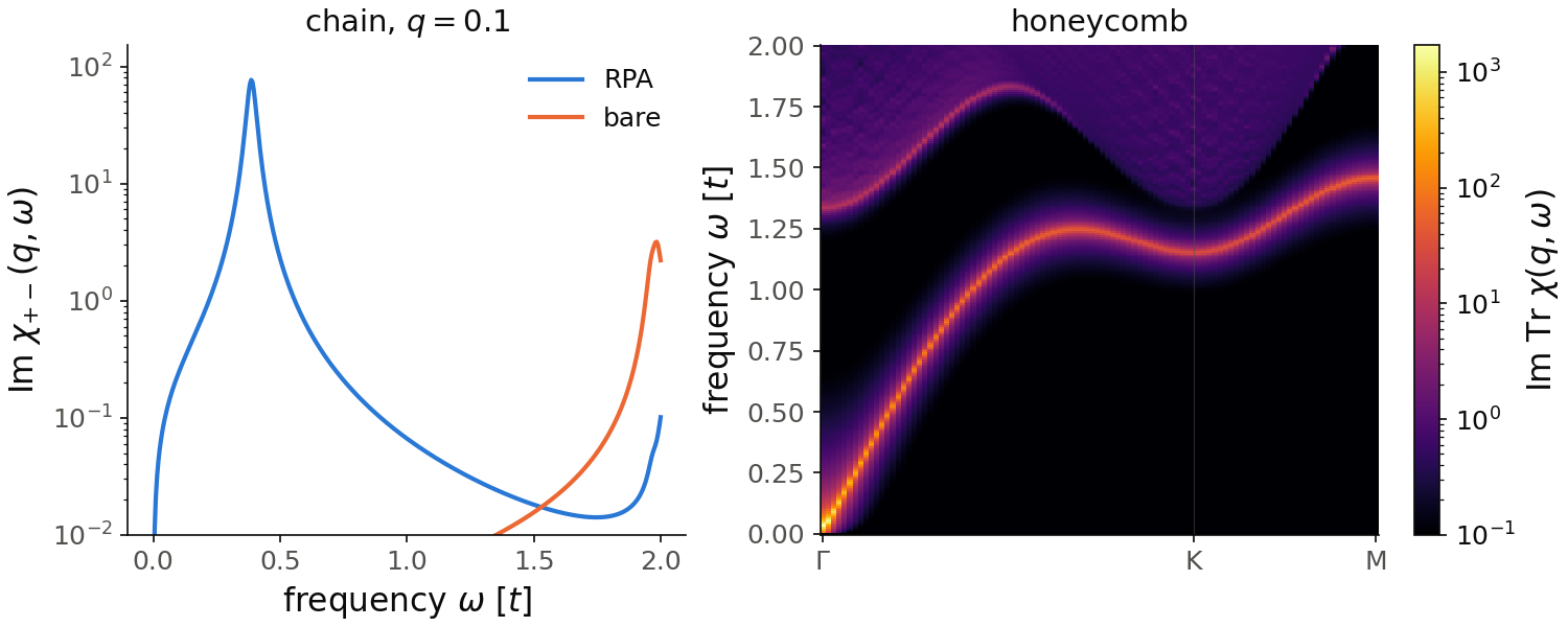
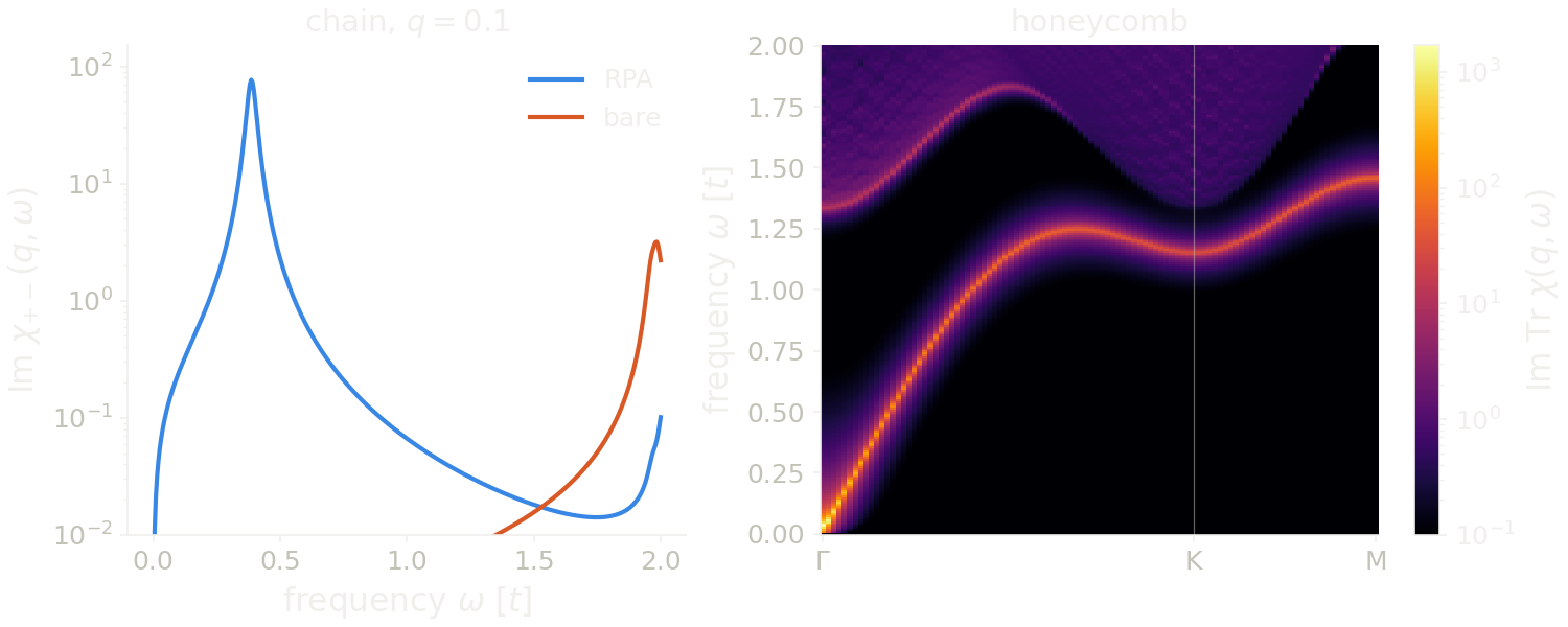
On the left is the first snippet, the chain at \(q=0.1\), with the bare response (RPA=False) added as a reference. Both are summed over the two sites of the cell and plotted on a log scale. The RPA response has one sharp peak, the magnon, at \(\omega=0.39t\). The bare response has no peak there: it has only the electron-hole continuum, which starts at the mean-field gap \(1.86t\) and peaks at \(2t\), with a tail below the gap from the broadening. With nk=80 instead of 40 the two curves do not change. On the right is qdisp of the honeycomb lattice, also on a log color scale. The bright line is the magnon. It starts at zero at \(\Gamma\), the Goldstone mode, rises to \(1.25t\) along \(\Gamma\)-K, is at \(1.16t\) at K and at \(1.45t\) at M. The weaker signal above it is the electron-hole continuum. It starts at about \(1.33t\) at \(\Gamma\) and at K, and its lower edge is a bright line. The magnon is the same with nk=30, 40 and 60; the larger nk only makes the continuum smoother, so we use nk=60.

Code of this figure (documentation/figures/spin_rpa.py)

from pyqula import geometry
import numpy as np
import style
from matplotlib.colors import LogNorm
g = geometry.bichain() # two sites per cell, so Neel order fits in the cell
h = g.get_hamiltonian(has_spin=True)
seed = h.copy() ; seed.add_antiferromagnetism(0.5) # symmetry-breaking seed
hmf = h.get_mean_field_hamiltonian(U=3.0,filling=0.5,mf=seed,nk=100) # magnetic state
(es,chis) = hmf.get_spinchi_ladder(energies=np.linspace(0.,2.,400),q=[0.1,0.,0.],nk=40,delta=2e-2)
(es,chi0) = hmf.get_spinchi_ladder(energies=np.linspace(0.,2.,400),q=[0.1,0.,0.],nk=40,delta=2e-2,
                                   RPA=False) # the bare response, as a reference

g2 = geometry.honeycomb_lattice() # already two sublattices per cell
h2 = g2.get_hamiltonian(has_spin=True)
hmf2 = h2.get_mean_field_hamiltonian(U=3.0,filling=0.5,mf="antiferro")
qdisp = hmf2.get_qdos_iets(energies=np.linspace(0.,2.,250),qpath=["G","K","M"],nq=120,nk=60,delta=1e-2)
(qs,ws,chimap) = qdisp # q-points, frequencies, Im Tr chi(q,w)

def draw(ax, c):
    im_rpa = np.trace(chis, axis1=1, axis2=2).imag # sum over the two sites
    im_0 = np.trace(chi0, axis1=1, axis2=2).imag
    ax[0].semilogy(es, im_rpa, color=c.blue, label="RPA")
    ax[0].semilogy(es, im_0, color=c.orange, label="bare")
    ax[0].set_ylim(1e-2, 2*im_rpa.max())
    ax[0].set_xlabel(r"frequency $\omega$ [$t$]")
    ax[0].set_ylabel(r"Im $\chi_{+-}(q,\omega)$")
    ax[0].set_title("chain, $q=0.1$")
    ax[0].legend(loc="upper right")
    x = np.arange(len(chimap))
    im = ax[1].pcolormesh(x, ws, np.clip(chimap.T, 1e-1, None), cmap=c.cmap,
                          norm=LogNorm(vmin=1e-1), shading="nearest",
                          rasterized=True)
    style.colorbar(im, ax[1], r"Im Tr $\chi(q,\omega)$")
    iK = np.argmin(np.abs(qs[:,0,1]-2/3)) # K = (-1/3,2/3) on this path
    ax[1].set_xticks([0, iK, x[-1]], [r"$\Gamma$", "K", "M"])
    ax[1].axvline(iK, color=c.ink2, lw=0.6, alpha=0.5)
    ax[1].set_ylabel(r"frequency $\omega$ [$t$]")
    ax[1].set_title("honeycomb")

style.save(draw, "spin_rpa", npanels=2)

See examples/1d/rpa/main.py (RPA spin response against \(q\) for an antiferromagnetic chain), examples/2d/rpa_triangular/main.py and examples/2d/rpa_honeycomb/main.py (dispersion along a q-path), and examples/0d/rpa_island/main.py and examples/0d/rpa_finite_chain/main.py (real-space IETS maps) for runnable scripts, and the notebooks 09_rpa_beyond_onsite.ipynb and 10_rpa_collective_modes.ipynb in jupyter-notebooks/functionalities/interacting_mean_field_hamiltonians/.

Precision on a GPU

The RPA functions can run on a GPU, after gpu.set_gpu(True) (see GPU). On a GPU the sum of the bare response is done in single precision by default, which changes the bare response by about \(10^{-7}\). Close to a pole, where \(1-V\chi_0\) is almost singular, the RPA amplifies this error: next to the Goldstone mode of a Néel state the dressed response changes by a few parts in \(10^4\). If you need the response at a pole with more digits, use chi_prec="double":

from pyqula import geometry
from pyqula import gpu
import numpy as np
gpu.set_gpu(True) # run the GPU kernels of the package on the device
g = geometry.honeycomb_lattice() # two sites per cell
h = g.get_hamiltonian() # first-neighbor hopping
hmf = h.get_mean_field_hamiltonian(U=3.0,filling=0.5,mf="antiferro",nk=10) # Neel mean field
es = np.linspace(0.01,1.0,50) # frequencies
(es,chi) = hmf.get_spinchi_full(q=[0.2,0.,0.],nk=10,energies=es,delta=0.05,
               chi_prec="double") # the response in double precision

On the CPU the default is already double precision.

Collective modes and magnon bands

The RPA response diverges when the matrix \(1-V(q)\chi_0(q,\omega)\) becomes singular. The frequencies where this happens are the collective modes: magnons in the spin channel, plasmons in the charge channel. If an eigenvalue of the kernel crosses zero already at \(\omega=0\), the state is unstable (a Stoner or charge-order instability). h.get_rpa_kernel_poles() scans a frequency window at fixed \(q\) and returns all the poles, for any pair of operators A, B and any interaction matrix V. By default it uses the charge channel and \(q=0\):

from pyqula import geometry
import numpy as np
g = geometry.bichain() # two sites per cell, so Neel order fits in the cell
h = g.get_hamiltonian()
seed = h.copy() ; seed.add_antiferromagnetism(0.5) # symmetry-breaking seed
hmf = h.get_mean_field_hamiltonian(U=3.0,nk=100,mf=seed,filling=0.5)
N = len(g.r) # the response matrix is one entry per site
V = 3.0*np.identity(N) # charge-channel interaction, in site space
poles = hmf.get_rpa_kernel_poles(V=V,q=[0.1,0.,0.],
        energies=np.linspace(0.,4.,200),delta=2e-2,nk=40)

V must have the size of the response matrix. In the charge channel there is one entry per site, so V is \(N\times N\). It is not hmf.V, the mean-field interaction in the space of sites and spins (\(2N\times2N\)), which gives a dimension error here. For the spin channel use h.get_magnon_bands() below, which builds the vertex from hmf.V itself.

poles is an array of shape (npoles,2), one row per mode: the frequency of the pole and the imaginary part of the kernel eigenvalue at the crossing. This imaginary part can have either sign, so look at its absolute value: a small value means a sharp mode, a large value means a damped mode or numerical noise. The snippet above gives three poles, between \(3.57t\) and \(3.88t\), all with an absolute value between 2.3 and 2.7, so they are all damped: in the charge channel this state has no sharp collective mode at \(q=0.1\).

Magnon bands

For the magnons, h.get_magnon_bands() finds the poles in the spin channel, between \(S_x\), \(S_y\) and \(S_z\), with the interaction of the converged mean field, along a q-path. The result is the magnon dispersion of the ordered state:

qs,ws,gammas = hmf.get_magnon_bands(nq=200,energies=np.linspace(0.01,3.,600),delta=2e-2,nk=80)

Each q-point can have a different number of poles, so qs, ws and gammas are flat arrays of the same length, ready for a scatter plot. qs is the index of the q-point along the path, as in h.get_bands(), ws the frequency of the pole and gammas its imaginary part; keep np.abs(gammas) < threshold to see only the sharp branches. For the antiferromagnetic chain you see an acoustic branch that goes to zero at \(q=0\), the Goldstone mode, and an optical branch above it.

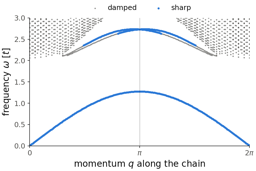
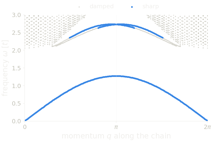
Here we keep the poles with \(|\gamma|<0.05\) as sharp. The acoustic branch goes from zero at \(q=0\) up to \(1.28t\) at \(q=\pi\), and back to zero at \(2\pi\). Above \(2.06t\) the gray points are damped poles, the electron-hole continuum. On a finite k-mesh the continuum is a set of discrete lines, and the poles between them make the regular pattern of gray points; a finer nk makes it denser, not smoother. The optical branch is the line of sharp points from \(2.35t\) to \(2.74t\), between \(q=\pi/2\) and \(3\pi/2\), inside the continuum. The two branches are converged: with nk=40 instead of 80 they move by less than \(10^{-3}t\). The scan takes about half a minute.

Code of this figure (documentation/figures/spin_magnons.py)

from pyqula import geometry
import numpy as np
import style
g = geometry.bichain() # two sites per cell, so Neel order fits in the cell
h = g.get_hamiltonian()
seed = h.copy() ; seed.add_antiferromagnetism(0.5) # symmetry-breaking seed
hmf = h.get_mean_field_hamiltonian(U=3.0,nk=100,mf=seed,filling=0.5)
qs,ws,gammas = hmf.get_magnon_bands(nq=200,energies=np.linspace(0.01,3.,600),delta=2e-2,nk=80)
sharp = np.abs(gammas) < 0.05 # sharp modes, the others are damped

def draw(ax, c):
    ax.scatter(qs[~sharp], ws[~sharp], s=2, color=c.ink2, alpha=0.5,
               label="damped")
    ax.scatter(qs[sharp], ws[sharp], s=6, color=c.blue, label="sharp")
    style.kpath(ax, qs, ["0", r"$\pi$", r"$2\pi$"])
    ax.set_xlabel("momentum $q$ along the chain")
    ax.set_ylabel(r"frequency $\omega$ [$t$]")
    ax.set_ylim(0, 3)
    ax.legend(loc="lower center", bbox_to_anchor=(0.5, 1.0), ncol=2)

style.save(draw, "spin_magnons")

See examples/1d/magnon_bands/main.py for a runnable script.

Interactions beyond onsite

The interaction V of get_rpa_kernel_poles can also have a range. It is then given as a dictionary {(n1,n2,n3): matrix}, with the key the lattice vector between the two unit cells, as for the hoppings in h.get_hopping_dict(). It is Fourier transformed in the same way as a hopping,

\[V(q) = \sum_{\mathbf R} V(\mathbf R)\, e^{2\pi i\, q\cdot \mathbf R},\]

with \(q\) in units of the reciprocal lattice vectors. For a first-neighbor \(V_1\) on a chain this gives \(V(q) = 2V_1\cos 2\pi q\), repulsive at \(q=0\) and attractive at the zone boundary \(q=1/2\):

import numpy as np
from pyqula import geometry
g = geometry.chain()
h = g.get_hamiltonian(has_spin=False)
N = h.intra.shape[0] # one site per cell here
I = np.identity(N)
V = {(0,0,0): 0.0*I, (1,0,0): 0.6*I, (-1,0,0): 0.6*I} # nearest-neighbor V1
poles = h.get_rpa_kernel_poles(V=V,q=[0.5,0.,0.],energies=np.linspace(0.,2.,60),
                                delta=2e-2,nk=200)

By default this is the charge channel, so V here is a density-density interaction, one entry per site. At \(q=1/2\) the snippet gives three poles, at \(0.011t\), \(0.081t\) and \(0.106t\). The lowest one, almost at zero frequency and with a small imaginary part (0.03), is the soft charge mode: the half-filled chain with this \(V_1\) is close to a charge-density-wave instability.

Which magnon method

In the spin channel, an interaction between different sites needs more care. We write the interaction as \(H_{\rm int} = \tfrac12\sum_{ij} V_{ij}\, n_i n_j\). In the transverse channel, the electron-hole pair \((i,j)\) with the electron on site \(i\) and the hole on site \(j\) is scattered by \(-V_{ij}\), the Fock (exchange) term, so the vertex is diagonal in the pair index \((i,j)\), not in the site index. An onsite \(U\) only has pairs with \(i=j\), and then a vertex with one index per site is exact. A neighbor interaction \(V_{ij}\) acts on pairs with \(i\neq j\), which a vertex with one index per site does not contain. For example, a ferromagnetic chain ordered only by \(V_1\) would have no magnon at all with a site vertex. For this reason the spin response functions (get_spinchi_full, get_spinchi_ladder, get_iets_ldos, get_magnon_bands) use the site vertex only for an onsite \(U\), and sum the series in the pair basis for any interaction between different sites. The call is the same in both cases. The pair basis does not support Nambu Hamiltonians.

h.get_magnon_bands() takes a method keyword with three options:

interaction	"rpa"	"pair"	"tdhf"
onsite Hubbard \(U\)	yes	yes	yes
neighbour-shell density-density \(V_1,V_2,\dots\)	through the pair basis	yes	yes
exchange \(J_1,J_2,\dots\) (isotropic or anisotropic)	through the pair basis	yes	yes
metallic reference	yes	yes	with metal=True
non-collinear (canted, spiral) state	yes	yes	yes
frequency-resolved \(\chi(\omega)\)	yes	yes	no (an eigenproblem)

• "rpa" (default): poles of the RPA kernel on a frequency grid. Exact for an onsite \(U\); for anything else it uses the pair basis.
• "pair": the same series in the pair basis. Only the pairs that the interaction connects enter, so a short-range interaction is cheap. It works for metals, and for any spin structure.
• "tdhf": time-dependent Hartree-Fock, an eigenvalue problem with no frequency grid and no broadening (see below).

"pair" and "tdhf" agree for every interaction in the table, and for an onsite \(U\) "rpa" gives the same magnons. This is true also at \(Q=\Gamma\). There the Goldstone mode has zero energy, and "pair" and "rpa" find it at an energy equal to the broadening delta, because the broadening moves it there. The list of "rpa" also has poles of the longitudinal \(S_z\) response, because it uses the full \((S_x,S_y,S_z)\) response. They are close to the ones that "pair" gives with channel="all". For a collinear state "pair" keeps only the spin-flip pairs, so it gives the magnons and not the charge and longitudinal excitations. With channel="all" it keeps all the pairs and gives those excitations too. As an example, the honeycomb lattice with an onsite \(U\) and a first-neighbor \(V_1\), its magnons and its transverse response:

import numpy as np
from pyqula import geometry
from pyqula.meanfield import VJinteraction
nk = 24                                 # the SCF and the magnon share this mesh
g = geometry.honeycomb_lattice()
hmf = VJinteraction(g.get_hamiltonian(),U=3.0,V1=0.5,filling=0.5,
                     mf="antiferro",nk=nk,mix=0.5,maxerror=1e-10).hamiltonian
qs,ws,gammas = hmf.get_magnon_bands(method="pair",nq=90,
                    energies=np.linspace(1e-3,3.,400),delta=1e-3,nk=nk)
es,chi = hmf.get_transverse_spinchi(energies=np.linspace(0.,2.,300),
                    q=[0.1,0.,0.],delta=1e-2,nk=nk)   # (Sx,Sy,Sz) x site chi(w)

The kernel has an exchange (Fock) term and a Hartree term. For a collinear state the Hartree term does not enter the transverse response. For a non-collinear state the spin sectors mix, and without the Hartree term the spin-rotation symmetry is broken and the acoustic magnon gets a wrong gap. Both terms are kept, so the Goldstone mode is at zero also for canted and spiral states.

An exchange interaction \(J\,\vec S_i\cdot\vec S_j\) is not a density-density interaction. Its Ising part \(J S^z_iS^z_j\) is, but its transverse part \(\tfrac{J}{2}(S^+_iS^-_j+{\rm h.c.})\) flips a spin on each site. The mean field writes \(S^x_iS^x_j\) and \(S^y_iS^y_j\) as Ising terms in two rotated spin frames, and records the three spin channels on the Hamiltonian it returns. "pair" and "tdhf" read these channels, so they include the transverse part, and for an isotropic \(J\) the Goldstone mode is at zero. This needs a Hamiltonian from VJinteraction, or from h.get_mean_field_hamiltonian() with J1, J2, J3 or Jr. The single-axis couplings SzSz, SxSx and SySy are recorded as an anisotropic exchange. A global spin rotation keeps an isotropic exchange, but would turn an anisotropic one into cross terms like \(S^x_iS^y_j\), so h.global_spin_rotation() refuses it (unless the rotation is around the axis of a uniaxial exchange); rotate the Hamiltonian before the mean-field calculation instead.

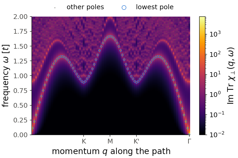
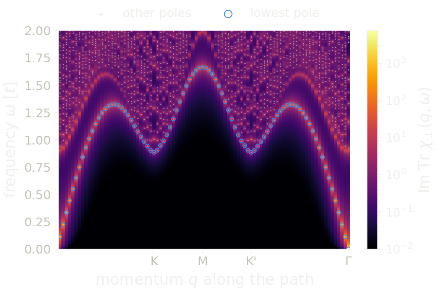
For the map we call hmf.get_transverse_spinchi() at 90 q-points of the default path, which goes from next to \(\Gamma\) through K, M and K' back to \(\Gamma\), and plot the trace of its imaginary part on a log color scale. The circles are the lowest pole from get_magnon_bands at each q-point, and the small gray dots are all the other poles. The lowest bright line is the magnon: \(0.11t\) at the first point of the path, \(0.89t\) at K and \(1.67t\) at M, and the circles sit on it. At \(q=(0.1,0,0)\), the call of the snippet, the magnon peak of the response is at \(0.57t\). At \(\Gamma\), on the right edge, the response is large at \(\omega\to0\), the Goldstone mode, and the pole scan lists it at \(\omega=10^{-3}\), the broadening delta. Above the magnon is the electron-hole continuum, which starts at about \(0.9t\) to \(1t\) near \(\Gamma\) and K. On a finite k-mesh it is a set of discrete lines, and the interaction shifts each line that it couples into a pole, so the scan lists between 60 and 130 poles at each q-point, the gray dots. They are not other collective modes. A bare line that the interaction does not couple is not a pole: there the kernel goes through infinity, not through zero, so it is not listed.

The mean field and the response use nk=24. For this state the error of the self-consistent loop goes down slowly with the default mixing mix=0.3, so we take mix=0.5. Then maxerror=1e-10 is reached in about 200 iterations. With nk=18 the magnon moves by at most \(0.015t\), near K, and with nk=30 it is at \(0.89t\) at K too. The coarse mesh nk=6 gives a magnon that is wrong by up to \(0.4t\) and a continuum of a few separate lines. The figure takes about five minutes.

Code of this figure (documentation/figures/spin_pair.py)

import numpy as np
import style
from matplotlib.colors import LogNorm
from pyqula import geometry
from pyqula.meanfield import VJinteraction
nk = 24                                 # the SCF and the magnon share this mesh
g = geometry.honeycomb_lattice()
hmf = VJinteraction(g.get_hamiltonian(),U=3.0,V1=0.5,filling=0.5,
                     mf="antiferro",nk=nk,mix=0.5,maxerror=1e-10).hamiltonian
qs,ws,gammas = hmf.get_magnon_bands(method="pair",nq=90,
                    energies=np.linspace(1e-3,3.,400),delta=1e-3,nk=nk)
es,chi = hmf.get_transverse_spinchi(energies=np.linspace(0.,2.,300),
                    q=[0.1,0.,0.],delta=1e-2,nk=nk)   # (Sx,Sy,Sz) x site chi(w)

# the same response along the path of the magnon bands, as a map
nq = 90
qpath = g.get_kpath(None,nk=nq) # the default path, from Gamma through K, M, K' to Gamma
chimap = [np.trace(hmf.get_transverse_spinchi(energies=es,q=q,delta=1e-2,nk=nk)[1],
                   axis1=1,axis2=2).imag for q in qpath]
x = (np.arange(nq)+1)/nq # position along the path
lowest = np.array([ws[qs==i].min() for i in range(nq)]) # lowest pole at each q

def draw(ax, c):
    im = ax.pcolormesh(x, es, np.clip(np.array(chimap).T, 1e-2, None),
                       cmap=c.cmap, norm=LogNorm(vmin=1e-2),
                       shading="nearest", rasterized=True)
    style.colorbar(im, ax, r"Im Tr $\chi_\perp(q,\omega)$")
    ax.scatter((qs+1)/nq, ws, s=1, color=c.ink2, alpha=0.5, lw=0,
               label="other poles")
    ax.scatter(x, lowest, s=14, facecolors="none", edgecolors=c.blue,
               lw=0.8, label="lowest pole")
    ax.set_xticks([1/3, 1/2, 2/3, 1], ["K", "M", "K'", r"$\Gamma$"])
    ax.set_xlabel("momentum $q$ along the path")
    ax.set_xlim(0.5/nq, 1+0.5/nq)
    ax.set_ylim(0, 2)
    ax.set_ylabel(r"frequency $\omega$ [$t$]")
    ax.legend(loc="lower center", bbox_to_anchor=(0.5, 1.0), ncol=2,
              markerscale=2)

style.save(draw, "spin_pair")

See jupyter-notebooks/functionalities/interacting_mean_field_hamiltonians/19_magnons_pair_ladder.ipynb for an executed notebook that compares the pair basis with time-dependent Hartree-Fock.

Magnons from time-dependent Hartree-Fock

You can think of a magnon as an exciton of a mean-field state: a bound electron-hole pair, where the electron and the hole have opposite spin. So the Bethe-Salpeter equation of Excitons, restricted to the spin-flip pairs, describes it. This is method="tdhf", time-dependent Hartree-Fock. It works in the pair basis, so it includes interactions between neighbors:

import numpy as np
from pyqula import geometry
from pyqula.meanfield import VJinteraction
nk = 24                                 # the SCF and the magnon share this mesh
g = geometry.honeycomb_lattice()
scf = VJinteraction(g.get_hamiltonian(),U=3.0,V1=0.5,filling=0.5,
                     mf="antiferro",nk=nk,mix=0.5,maxerror=1e-10)
hmf = scf.hamiltonian
print(hmf.get_goldstone_residual(nk=nk))          # 3e-10: zero to the SCF tolerance
qs,es = hmf.get_magnon_bands(method="tdhf",nk=nk,nq=90,n=2)

qs and es are flat arrays, as for "rpa", with qs the index along the q-path. Without qpath, the path on the honeycomb lattice is the line from \((0,0)\) to \((1,1)\) in units of the reciprocal lattice vectors, so it goes \(\Gamma\), K, M, K', \(\Gamma\), and its first point is next to \(\Gamma\), not \(\Gamma\) itself. es is complex when the mean-field state is unstable against some excitation. h.get_magnon_energies(Q=...) gives the magnon energies at a single momentum.

The Goldstone theorem is the check. A magnetic state without spin-orbit coupling breaks the spin-rotation symmetry, so a uniform rotation of all the spins costs no energy, and there is a magnon at exactly zero energy at \(Q=0\). h.get_goldstone_residual() measures the distance from this. It is proportional to the tolerance of the mean-field calculation, about \(3\times10^{-10}\) for maxerror=1e-10, so check it before reading any dispersion. A small imaginary part of the same size on the acoustic branch is expected.

Three things matter:

• The mean field and the magnons must use the same nk. A mean field converged at nk=20 is not self-consistent on a mesh of nk=4, and then the acoustic magnon gets a large wrong gap. The Hamiltonian does not keep the mesh it was converged on, so check with get_goldstone_residual.
• A metal needs metal=True. By default the same number of bands is taken as occupied at every k-point, which is wrong for a metal. With metal=True the occupied states are chosen at each k-point, which is what an itinerant magnet needs; for an insulator it changes nothing. In a metal the magnon is inside the Stoner continuum and is not the lowest mode, so use by="weight" to select the branches by their spin weight instead of by energy. Also, \(E(q)=E(-q)\) only if the occupied states are symmetric under \(k\to-k\) on the mesh, so choose a mesh with this symmetry.
• An isotropic exchange (J1, J2, J3, Jr) from the mean field has its transverse part and its Goldstone mode. A hand-built exchange matrix has only the Ising part and no record of its channels, so it raises ValueError (with it, the magnon would get a wrong gap of order \(J\)). An anisotropic exchange (J1x, J1y, J1z not equal, or SzSz, SxSx, SySy) breaks the spin-rotation symmetry, so its magnon gap is physical and there is no Goldstone mode to check; it also raises ValueError, and check_su2=False computes its spectrum.

For a collinear state only the spin-flip pairs are needed, which is exact and cheaper, and this is the default. For a canted or spiral state all the pairs are used automatically (channel="all" forces it). This includes the 120-degree spiral of the triangular-lattice Hubbard model, whose Goldstone mode is at zero to the tolerance of the mean field. For an onsite \(U\), where both are exact, "tdhf" and "rpa" give the same magnons.

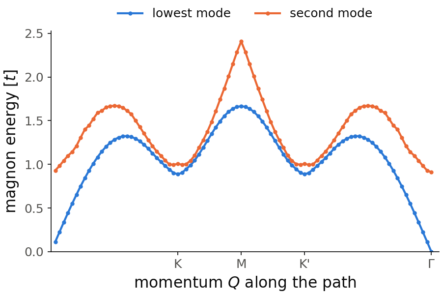
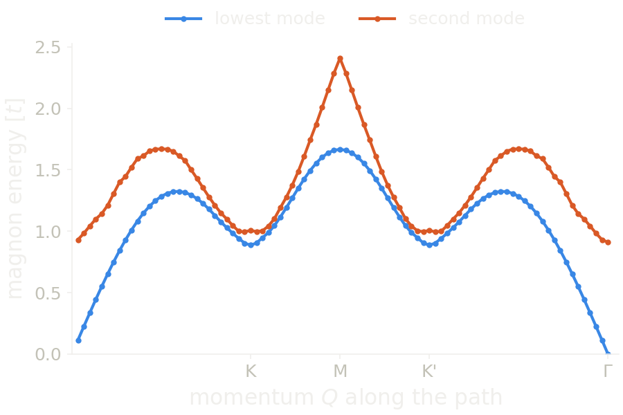
The Goldstone residual is \(3\times10^{-8}\), so the dispersion can be read. The path starts next to \(\Gamma\), not at it, and ends at \(\Gamma\). There the lowest mode is at zero, the Goldstone mode, and the second one is at \(0.91t\). At K the lowest mode is at \(0.89t\), and at M the two modes are at \(1.67t\) and \(2.41t\). The lowest mode has the same energies as the lowest poles of the pair-basis map above, to \(10^{-3}t\), as it should be. Both branches are smooth along the path with nk=24. On a coarse mesh, such as nk=6, they zigzag between neighboring \(Q\), because the electron-hole pairs of the mesh at \(k\) and \(k+Q\) change from one \(Q\) to the next. The lowest mode is converged: it moves by at most \(0.015t\) from nk=18 to 24, and by \(0.005t\) at K from nk=24 to 30. The second mode near K and K' is the bottom of the electron-hole continuum, not a second magnon, and it converges more slowly: at K it is at \(1.09t\), \(1.01t\) and \(0.97t\) for nk=18, 24 and 30. Its limit is the bottom of the continuum at K, the smallest \(E_c(\mathbf k+\mathbf Q)-E_v(\mathbf k)\) of the mean-field bands, which is \(0.91t\), the mean-field gap, since the valence band has its maximum at K and the conduction band its minimum at K'. On a finite mesh the lowest pair state sits above this edge and comes down to it only slowly as nk grows, so the second mode is a discrete level of the continuum and not a converged branch. The magnon at K, \(0.89t\), is just below the edge. The figure takes about eight minutes.

Code of this figure (documentation/figures/spin_tdhf.py)

import numpy as np
import style
from pyqula import geometry
from pyqula.meanfield import VJinteraction
nk = 24                                 # the SCF and the magnon share this mesh
g = geometry.honeycomb_lattice()
scf = VJinteraction(g.get_hamiltonian(),U=3.0,V1=0.5,filling=0.5,
                     mf="antiferro",nk=nk,mix=0.5,maxerror=1e-10)
hmf = scf.hamiltonian
print(hmf.get_goldstone_residual(nk=nk))          # 3e-10: zero to the SCF tolerance
qs,es = hmf.get_magnon_bands(method="tdhf",nk=nk,nq=90,n=2)
x = (np.arange(90)+1)/90 # position along the path, from Gamma through K, M, K' to Gamma
E = np.sort(es.real.reshape(90,2), axis=1) # two branches at each q
print(E[[0,29,44,89]]) # first point, K, M and Gamma

def draw(ax, c):
    ax.plot(x, E[:,0], "o-", ms=3, color=c.blue, label="lowest mode")
    ax.plot(x, E[:,1], "o-", ms=3, color=c.orange, label="second mode")
    ax.set_xticks([1/3, 1/2, 2/3, 1], ["K", "M", "K'", r"$\Gamma$"])
    ax.set_xlim(0, 1.02)
    ax.set_ylim(0, None)
    ax.set_xlabel("momentum $Q$ along the path")
    ax.set_ylabel(r"magnon energy [$t$]")
    ax.legend(loc="lower center", bbox_to_anchor=(0.5, 1.0), ncol=2)

style.save(draw, "spin_tdhf")

See examples/2d/magnon_bands_tdhf/main.py for a runnable script, and jupyter-notebooks/functionalities/interacting_mean_field_hamiltonians/18_magnons_tdhf.ipynb for an executed notebook.

Charge response and plasmons

The same RPA can be done in the charge channel, with h.get_densitychi_RPA() and h.get_plasmon_bands(). These are the density-density versions of get_spinchi_full and get_magnon_bands. The collective modes are now plasmons, or the modes of a charge order. The interaction is a density-density interaction with an onsite U, neighbor shells V1, V2, V3, and a general Vr(r), as in Vinteraction and VJinteraction. Different from the spin channel, the interaction is given as keywords and is not read from h.V, so no mean-field calculation is needed: the bare response of the Hamiltonian you give is dressed with this interaction. This Hamiltonian can also be a converged mean-field one.

import numpy as np
from pyqula import geometry
g = geometry.chain()
h = g.get_hamiltonian(has_spin=True) # 1D chain at half filling
qs,ws,gammas = h.get_plasmon_bands(V1=0.6,qpath=[[0.3,0.,0.],[0.4,0.,0.],[0.5,0.,0.]],nq=3,
                                    energies=np.linspace(0.,1.,100),delta=2e-2,nk=2000)

qs, ws and gammas are as in get_magnon_bands. What matters here is the wavevector. At half filling the chain has perfect nesting at \(q=1/2\) (\(k=\pi\)), so the static charge response is large there. A repulsive V1 gives \(V(q)=2V_1\cos2\pi q<0\) at the zone boundary, so it pushes the charge channel toward an instability at \(q=1/2\), a charge-density wave. This is the charge version of the Stoner instability of the spin channel.

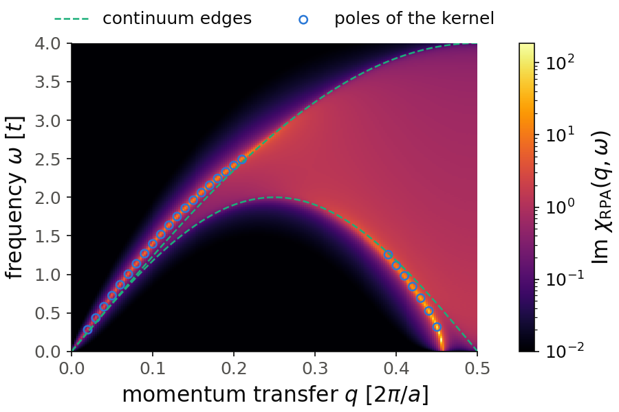
The map is not in the snippet: we call h.get_densitychi_RPA() with the same V1=0.6 at 201 values of \(q\) with nk=1000, and plot it on a log color scale. With nk=3000 the map is the same. The dashed lines are the edges of the free electron-hole continuum, \(2t\sin 2\pi q\) and \(4t\sin\pi q\). The circles are the poles of get_plasmon_bands at 50 values of \(q\), with energies from 0 to \(4t\). At small \(q\), where \(V(q)>0\), the RPA moves the weight to the upper edge and a little above it: this is the plasmon. Its poles go from \(0.28t\) at \(q=0.02\), just above the edge, to \(2.49t\) at \(q=0.21\), where it enters the continuum and the poles stop. Their \(|\gamma|\) is between 0.11 and 0.3 from \(q=0.04\) on, and 0.7 at \(q=0.02\), so the plasmon is damped most at the smallest \(q\). Near \(q=1/2\), where \(V(q)<0\), the weight moves to the lower edge and below it, toward zero frequency: this is the soft charge mode of the charge-density wave. Its poles go from \(1.26t\) at \(q=0.39\) down to \(0.32t\) at \(q=0.45\), below the edge, and they get sharper as the frequency goes down, \(|\gamma|=0.01\) at \(q=0.45\). Closer to \(q=1/2\) there is no pole. At \(q=1/2\) the real part of the kernel eigenvalue changes sign at \(0.60t\), but the eigenvalue stays at about 0.6 in absolute value, so the kernel never comes close to zero. The window of the snippet, energies from 0 to 1, misses the mode at \(q=0.4\), at \(1.115t\), just below the edge of the continuum at \(1.18t\); with energies up to \(2t\) the same call finds it. The figure takes about three and a half minutes.

Code of this figure (documentation/figures/spin_plasmon.py)

import numpy as np
import style
from matplotlib.colors import LogNorm
from pyqula import geometry
g = geometry.chain()
h = g.get_hamiltonian(has_spin=True) # 1D chain at half filling
qs,ws,gammas = h.get_plasmon_bands(V1=0.6,qpath=[[0.3,0.,0.],[0.4,0.,0.],[0.5,0.,0.]],nq=3,
                                    energies=np.linspace(0.,1.,100),delta=2e-2,nk=2000)

# the poles along the whole q-axis, with a window up to 4t
qpoles = np.linspace(0.01,0.5,50)
qp,wp,gp = h.get_plasmon_bands(V1=0.6,qpath=[[q,0.,0.] for q in qpoles],nq=len(qpoles),
                                    energies=np.linspace(0.,4.,400),delta=2e-2,nk=2000)
print(np.array([qpoles[qp.astype(int)],wp,np.abs(gp)]).T.round(3)) # q, frequency, |gamma|

# the RPA charge response over (q,omega), as a map
qmap = np.linspace(0.,0.5,201) # momentum transfer
es = np.linspace(0.,4.,300) # frequencies
chimap = [h.get_densitychi_RPA(V1=0.6,q=[q,0.,0.],energies=es,delta=2e-2,nk=1000)[1][:,0,0].imag
          for q in qmap]

def draw(ax, c):
    im = ax.pcolormesh(qmap, es, np.clip(np.array(chimap).T, 1e-2, None),
                       cmap=c.cmap, norm=LogNorm(vmin=1e-2),
                       shading="nearest", rasterized=True)
    style.colorbar(im, ax, r"Im $\chi_{\rm RPA}(q,\omega)$")
    qline = np.linspace(0., 0.5, 100)
    ax.plot(qline, 4*np.sin(np.pi*qline), "--", color=c.green, lw=1.2)
    ax.plot(qline, 2*np.sin(2*np.pi*qline), "--", color=c.green, lw=1.2,
            label="continuum edges")
    ax.scatter(qpoles[qp.astype(int)], wp, s=30, facecolors="none",
               edgecolors=c.blue, lw=1.2, label="poles of the kernel")
    ax.set_xlabel(r"momentum transfer $q$ [$2\pi/a$]")
    ax.set_ylabel(r"frequency $\omega$ [$t$]")
    ax.set_xlim(0, 0.5)
    ax.set_ylim(0, 4)
    ax.legend(loc="lower center", bbox_to_anchor=(0.5, 1.0), ncol=2)

style.save(draw, "spin_plasmon")