Exchange interactions

The interactions of Mean-field Hubbard models are of density-density type: they couple the charge on one site to the charge on another. In a magnet made of local moments the natural interaction is instead an exchange coupling between the spins of two sites. In this page we treat it at the mean-field level, alone or together with the density-density interactions. We also see what decides whether a self-consistent calculation converges, and how to treat large systems.

Spin-spin exchange

The exchange Hamiltonian is

\[ H_J = J_z\sum_{\langle ij\rangle} S^z_i S^z_j + J_x\sum_{\langle ij\rangle} S^x_i S^x_j + J_y\sum_{\langle ij\rangle} S^y_i S^y_j , \qquad \vec S_i = \frac{1}{2}\sum_{ss'} c^\dagger_{i,s}\vec\sigma_{ss'}c_{i,s'} , \]

where \(\vec S_i\) is the spin-1/2 operator of the electrons on site \(i\), \(\vec\sigma\) are the Pauli matrices, and each bond \(\langle ij\rangle\) is counted once. \(J>0\) is antiferromagnetic and \(J<0\) is ferromagnetic. With \(S^z_i=(n_{i,\uparrow}-n_{i,\downarrow})/2\) we get

\[ S^z_i S^z_j = \tfrac14\left( n_{i,\uparrow}n_{j,\uparrow} - n_{i,\uparrow}n_{j,\downarrow} - n_{i,\downarrow}n_{j,\uparrow} + n_{i,\downarrow}n_{j,\downarrow} \right), \]

so \(S^z_iS^z_j\) is a density-density interaction between spin-orbitals, and it is decoupled in the same way as \(U\) and \(V_1\), with all the Hartree and Fock terms. The \(S^x_iS^x_j\) and \(S^y_iS^y_j\) terms are the same after a rotation of the spin axis.

The methods are

• h.get_szsz_mean_field_hamiltonian(): the \(S^zS^z\) coupling only.
• h.get_sxsx_mean_field_hamiltonian(), h.get_sysy_mean_field_hamiltonian(): the same along \(x\) and \(y\).
• h.get_exchange_mean_field_hamiltonian(): different couplings along the three axes, an anisotropic exchange.
• h.get_combined_mean_field_hamiltonian(): exchange and density-density interactions together.

The couplings are J1, J2, J3 for first, second and third neighbors, and Jr for a general function of the two positions, in the same convention as V1, V2, V3 and Vr. Like Vr, Jr is evaluated on every pair of sites up to rcut, including the pair of a site with itself. So a coupling meant only for bonds must return zero at zero distance; a value \(J_r(0)\) is an onsite term \(\frac{1}{2}J_r(0)\,\vec S_i\cdot\vec S_i\), which at the mean-field level acts as a Hubbard \(U=-\frac{3}{4}J_r(0)\).

As an example, a ferromagnetic \(S^zS^z\) coupling on a chain away from half filling:

from pyqula import geometry
g = geometry.chain() # a chain, prone to ferromagnetic order away from half filling
h = g.get_hamiltonian(has_spin=True)
h = h.get_szsz_mean_field_hamiltonian(J1=-2.0,filling=0.2,
                                       mf="ferroZ", # ferromagnetic Sz-Sz coupling
                                       nk=10,mix=0.3,maxite=300)
m = h.get_magnetization() # uniform moment along z

The loop converges, and every site gets the same moment along \(z\), which h.get_magnetization() returns as one vector per site. But this moment is not a converged ferromagnet. It is \(-0.2\) with nk=10, \(-0.1\) with nk=20, \(-0.05\) with nk=40 and \(-0.02\) with nk=100, so it scales as \(2/n_k\): one electron on the k-mesh flips its spin, and the moment goes to zero for a fine mesh. So at \(J_1=-2\) the chain is not a ferromagnet at the mean-field level. A real ferromagnet needs a larger coupling and a stronger guess. With \(J_1=-6\), nk=40 and a guess with an exchange field of 1 instead of the 0.1 of "ferroZ", the loop converges to a fully polarized state, with moment \(-0.4\), and its total energy is lower than the one of the unpolarized solution. On a finer mesh, nk=60 or nk=100, this state needs a small temperature, T=0.01, for the reason given in the convergence section below. With the weak "ferroZ" guess the same \(J_1=-6\) still gives \(-0.05\), because the unpolarized state is also a self-consistent solution. In both cases the exchange field is found by the calculation, it is not added by hand with h.add_exchange().

Convergence

All the mean-field methods of this page and of Mean-field Hubbard models raise an error, MeanFieldConvergenceError, when the loop does not converge. Its message gives the number of iterations, the error reached and maxerror. In a sweep over a parameter, catch it with try and except to skip the points that do not converge. It is imported with from pyqula.meanfield import MeanFieldConvergenceError. The functions of pyqula.meanfield that run the loop directly, such as meanfield.VJinteraction(), raise the same error. With check_convergence=False they return the unconverged result instead, with .converged set to False. Four keywords control the convergence:

• nk (default 8): the number of k-points per direction used to compute the expectation values.
• mix (default 0.1): the fraction of the new mean field mixed into the old one at each iteration.
• maxite (default 1000): the maximum number of iterations; None means no limit.
• maxerror (default \(10^{-5}\)): the largest allowed change of the mean field between two iterations.

The k-mesh is usually the problem. If the mesh does not resolve the Fermi surface, the occupied states change from one iteration to the next, and no mixing helps. The chain above at filling=0.2 never converges with nk=8, and converges at once with nk=10. The reason is that it converges when the mesh holds a whole number of electrons, \(0.4\,n_k\), as for nk=10 and nk=15, and not for nk=8 or nk=12. So nk is the first thing to change. A smaller mix helps when the loop oscillates around a solution. A second problem appears when two states, at \(k\) and \(-k\), sit exactly at the Fermi level, as for the polarized chain at \(J_1=-6\) with nk=60 or nk=100. At the default temperature, \(T=10^{-7}\), a very small change of the mean field puts one of them below the Fermi level and the other one above. At the next iteration the two swap, so the loop oscillates forever and no mix helps. A small temperature, T=0.01 in units of the hopping, smooths the occupation of these two states, and the loop converges to the same state as at nk=40, with moment \(-0.4\) and the same energy per site within \(10^{-3}\). The same holds for h.get_combined_mean_field_hamiltonian(), for example with \(U=5\) and \(J_1=-1\) at nk=40. On a large system 1000 iterations take long, so a smaller maxite is useful while you explore parameters.

Anisotropic exchange

Different couplings along the three axes are given in one calculation with h.get_exchange_mean_field_hamiltonian(), here \(J_z=-1\) and \(J_x=-0.5\) on first neighbors:

h = g.get_hamiltonian(has_spin=True)
h = h.get_exchange_mean_field_hamiltonian(Jz1=-1.0,Jx1=-0.5,
                                            filling=0.2,mf="ferroZ",
                                            nk=10,mix=0.3,maxite=300)

As for \(S^zS^z\) above, the moment of this chain is \(-0.2\) with nk=10 and \(-0.05\) with nk=40, so it scales as \(2/n_k\) and is not a converged ferromagnet.

Exchange and density-density interactions together

A model with both charge and magnetic correlations needs density-density interactions and exchange together. h.get_combined_mean_field_hamiltonian() solves them in one self-consistent calculation. Its exchange keywords are

• J1, J2, J3, Jr: isotropic Heisenberg couplings \(J(S^x_iS^x_j+S^y_iS^y_j+S^z_iS^z_j)\) on the first, second and third neighbors, and as a function of the positions.
• J1x, J1y, J1z: an anisotropy added to J1 for first neighbors only, so the first-neighbor coupling along \(z\) is \(J_1+J_{1z}\).

All of them are zero by default, and U, V1, V2, V3, Vr are as in Mean-field Hubbard models.

h = g.get_hamiltonian(has_spin=True)
h = h.get_combined_mean_field_hamiltonian(U=5.0,J1=-1.0,
                                            filling=0.2,mf="ferroZ")

This snippet runs with the default nk=8 and gives a moment of \(-0.375\), and with nk=40 it gives \(-0.05\), again \(2/n_k\). So on this chain it shows how to call the method, not a converged ordered state. With nk=100, or with \(U=10\) or \(J_1=-3\) at nk=40, the loop does not converge.

Superconductivity from exchange

All the exchange methods also work on a Bogoliubov-de Gennes (BdG) Hamiltonian, after h.turn_nambu() or h.setup_nambu_spinor(). Then the exchange is decoupled in the normal and in the anomalous channels, as \(U\) and \(V_1\) are. So exchange alone can give superconductivity. An antiferromagnetic isotropic \(J\), without any \(U\) or \(V\), can decouple into a singlet paired state: this is the resonating-valence-bond mechanism of exchange-driven superconductivity. A ferromagnetic \(J\) does not do this and stays magnetic. This paired state must be seeded: pass as mf a Hamiltonian with a small pairing, for example with h.add_swave(0.1). A random guess has little overlap with it and usually goes back to zero pairing.

A state with both magnetic and superconducting order can come from an exchange field together with an attractive \(V_1\):

h = g.get_hamiltonian(has_spin=True)
h.add_exchange([0.,0.,0.3])
h.turn_nambu()
h = h.get_combined_mean_field_hamiltonian(V1=-1.0,J1z=-0.3,
                                            filling=0.3,mf="random")

With the default nk=8 this result is not converged in the k-mesh: one run gave a gap of only 0.02 in the BdG bands, and another run did not converge. With nk=20 and nk=40 the gap is 0.14 and 0.15, and the moment is \(-0.14\) and \(-0.15\), so here a k-mesh of at least nk=20 gives a state with both magnetic and superconducting order.

With return_total_energy=True the method also returns the mean-field total energy, with the double counting of both the normal and the pairing mean field removed. Comparing this energy with the one of an unpaired solution of the same interaction tells you which of the two is the ground state at the mean-field level.

Nonlinear solvers

If a loop does not converge with plain mixing, it can be solved with a nonlinear solver instead, with use_jax=True. One iteration of the loop is a map \(x\to f(x)\) of the mean field, and the solver looks for the root of \(x-f(x)=0\). solver="error_gradient" is the most robust on a generic Hamiltonian and the first one to try; "newton" is the default. The other options are "newton_krylov", "fsolve", "lbfgs", "broyden_mixing" and "linear_mixing". These solvers work only for the normal state, and do not accept constrains.

h = g.get_hamiltonian(has_spin=True)
h = h.get_combined_mean_field_hamiltonian(U=5.0,J1=-1.0,filling=0.2,
                                            mf="ferroZ",use_jax=True,
                                            solver="newton")

Expectation values from the kernel polynomial method

At each iteration the expectation values come from diagonalizing the Bloch Hamiltonian at every k-point, and for a large system this is the expensive step. With integration="kpm" the density matrix is computed instead with a Chebyshev expansion, the kernel polynomial method, without any diagonalization:

h = g.get_hamiltonian(has_spin=True)
h = h.get_combined_mean_field_hamiltonian(U=5.0,J1=-1.0,filling=0.2,
                                            mf="ferroZ",integration="kpm")

The expansion with npol polynomials resolves energies down to roughly the bandwidth divided by npol. A magnetic splitting or a superconducting gap smaller than this is smeared out. In practice the resolution should be several times smaller than the gap, and about ten times smaller close to a transition, where a gapped and a gapless solution have almost the same energy. When a model has several self-consistent states, this route and exact diagonalization can converge to different ones from the same guess. Keep the one with the lower total energy.

On a GPU

The same calculation can run on a GPU (see GPU). There kpm_prec sets the precision. Single precision, the default on the GPU, changes the density matrix by about \(10^{-8}\), much less than a finite npol does, but the change of the mean field between iterations then stops at about \(10^{-6}\). For a maxerror below this, use kpm_prec="double".

from pyqula import gpu
gpu.set_gpu(True)
h = g.get_hamiltonian(has_spin=True)
h = h.get_combined_mean_field_hamiltonian(U=5.0,J1=-1.0,filling=0.2,
                                            mf="ferroZ",integration="kpm",
                                            npol=400,kpm_prec="single")

gpu.set_gpu(False) returns the rest of the script to the CPU.

Large islands

For a large finite island, say \(10^5\) sites, a dense Hamiltonian does not fit in memory. Build it sparse, with is_sparse=True. Then the interaction, the density matrix and the mean field stay sparse during the whole loop, and the memory grows linearly with the number of sites. This works with spin-orbit coupling, with exchange, and with the Nambu basis of a superconductor:

from pyqula import geometry
g = geometry.honeycomb_lattice().get_supercell(12) # a honeycomb island
g.dimensionality = 0 # make it finite
h = g.get_hamiltonian(has_spin=True,is_sparse=True) # keep the matrices sparse
h.add_rashba(0.2) # spin-orbit coupling, so the moments are not collinear
h = h.get_mean_field_hamiltonian(U=3.0,filling=0.5,mf="random",
                                  integration="kpm",npol=150,mix=0.5,
                                  maxerror=1e-3)

The result is the same self-consistent Hamiltonian as with a dense matrix, and it is still sparse, so h.extract("mx") and similar read the exchange field site by site without any diagonalization. Some points to keep in mind:

• maxerror is the change of the mean field per entry, for any size of the island. The direction of the moments, which the Rashba coupling selects only weakly, relaxes slowly. The snippet reaches a change of \(10^{-3}\) in less than a hundred iterations, while \(2\times10^{-4}\) takes about 400.
• The total energy is the band energy of the KPM density matrix at zero temperature, \(\mathrm{Tr}(H\rho)\). It tends to the sum of the occupied levels as npol grows.
• On an island, Vr and Jr need an explicit rcut, otherwise every pair of sites interacts.
• On a small island, if the filling times the number of states is not an integer, KPM keeps the fractional number of electrons, while exact diagonalization rounds it to whole states. So the two converge to slightly different states.

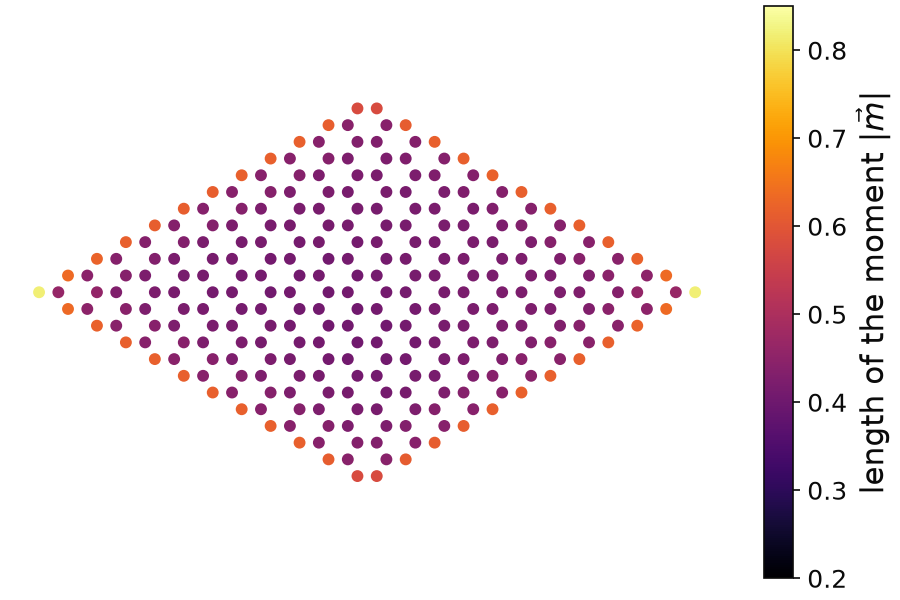
The map shows the length of the moment on each of the 288 sites of the island. In the bulk it is about \(0.42\). On the zigzag edges, where a site has two neighbors instead of three, it grows to about \(0.62\), and on the two corner sites, with one neighbor, it is \(0.82\). The moment of every site is antiparallel to the ones of its neighbors, so this is the antiferromagnet of the honeycomb lattice, and its direction changes across the island because of the Rashba coupling. Spin-polarized STM would see the larger moments at the edges.

Code of this figure (documentation/figures/exchange_island.py)

import numpy as np
import style
from pyqula import geometry
np.random.seed(1) # the same random guess in every run
g = geometry.honeycomb_lattice().get_supercell(12) # a honeycomb island
g.dimensionality = 0 # make it finite
h = g.get_hamiltonian(has_spin=True,is_sparse=True) # keep the matrices sparse
h.add_rashba(0.2) # spin-orbit coupling, so the moments are not collinear
h = h.get_mean_field_hamiltonian(U=3.0,filling=0.5,mf="random",
                                  integration="kpm",npol=150,mix=0.5,
                                  maxerror=1e-3)
m = np.linalg.norm(h.get_magnetization(),axis=1) # length of the moment of each site

def draw(ax, c):
    sc = ax.scatter(g.r[:,0], g.r[:,1], c=m, s=22, cmap=c.cmap, vmin=0.2, vmax=0.85)
    style.colorbar(sc, ax, r"length of the moment $|\vec m|$")
    ax.set_aspect("equal")
    ax.axis("off")

style.save(draw, "exchange_island")

See examples/0d/kpm_scf_sparse/main.py for a runnable script with an antiferromagnet and a superconductor.

Truncation to a radius

The time of one iteration grows as the square of the number of sites, because the occupation of each orbital comes from a Chebyshev recursion over the whole island. But after \(n\) steps of the recursion, a vector that starts on one orbital has only reached the sites within \(n\) hops. So we can compute the occupations around an orbital with the Hamiltonian restricted to the sites within \(R\) hops: this is exact up to the moment \(2R\). Whether this is enough depends on the physics. In a gapped state the density matrix decays exponentially, over a length of the order of the velocity divided by the gap (or by the temperature at finite temperature), so the error falls exponentially with \(R\). In a metal at zero temperature the density matrix decays as a power law, and the truncation is not controlled. kpm_radius sets \(R\), in hops between sites:

h = g.get_hamiltonian(has_spin=True,is_sparse=True) # the same island
h.add_rashba(0.2)
h = h.get_mean_field_hamiltonian(U=3.0,filling=0.5,mf="random",
                                  integration="kpm",npol=150,mix=0.5,
                                  maxerror=1e-3,kpm_radius=8)

The cost of an iteration is now linear in the number of sites. Converge \(R\) as you converge a k-mesh, by comparing two values. For the antiferromagnet of a half-filled honeycomb island at \(U=3\), the exchange field differs from the one of the full recursion by 0.11, 0.023, 0.005 and 0.001 at 2, 4, 6 and 8 hops, so every two hops reduce the error by a factor of about five. On six desktop cores, one iteration of the Hubbard model with Rashba coupling on a square island of \(10^5\) sites takes about half a minute with kpm_radius=10 and npol=100, and about two minutes with the Nambu basis of a superconductor.

See the notebooks 03_spin_spin_exchange.ipynb, 11_kpm_scf.ipynb and 12_jax_scf_solvers.ipynb in jupyter-notebooks/functionalities/interacting_mean_field_hamiltonians/ for executed versions.