Charge and generic response functions

In this page we compute the bare response function of a single-particle Hamiltonian: first the charge response, then the response of any pair of operators, and finally the RKKY coupling between two magnetic moments, which is a static response.

Charge-charge response function

We put a small potential on site \(j\) and look at the change of the density on site \(i\). This is the charge-charge response function, computed with h.get_chi(). For a periodic system at momentum transfer \(q\) it is the Lindhard function

\[ \chi_{ij}(q,\omega) = \frac{1}{N_k}\sum_{\mathbf k}\sum_{n,m} \left[f(\epsilon_{\mathbf k,n}) - f(\epsilon_{\mathbf k+q,m})\right] \frac{ \Psi^*_{\mathbf k,n}(i)\,\Psi_{\mathbf k+q,m}(i)\; \Psi^*_{\mathbf k+q,m}(j)\,\Psi_{\mathbf k,n}(j) } { \epsilon_{\mathbf k,n} - \epsilon_{\mathbf k+q,m} - \omega + i\delta } , \]

where \(\Psi_{\mathbf k,n}(i)\) is the amplitude of the eigenstate \(n\) at momentum \(\mathbf k\) on site \(i\) (summed over spin), \(\epsilon_{\mathbf k,n}\) its energy, \(f\) the Fermi-Dirac distribution and \(\delta\) a broadening. A pair of states contributes only if one is occupied and the other is empty, and it resonates at the energy difference of the two states. A transition from an occupied state to an empty state at energy \(\omega\) above gives a positive \(\mathrm{Im}\,\chi_{ii}\) at \(\omega>0\), and a negative one at \(\omega<0\). The static limit is negative: a positive potential pushes electrons away.

h.get_chi() returns \(\chi_{ii}(q,\omega)\) averaged over the sites \(i\) of the unit cell. For the chain at \(q=0\):

from pyqula import geometry
g = geometry.chain() # create a chain
h = g.get_hamiltonian() # create hamiltonian of the system
(es,chis) = h.get_chi(q=[0.,0.,0.]) # get response function

es contains the frequencies and chis one complex number per frequency. The imaginary part is what inelastic scattering (electron energy loss, inelastic x-rays) measures. At \(q=0\) the chain has a single band, so there is no other state at the same momentum to scatter into, and the response vanishes at any finite frequency. Only the static limit survives,

\[\chi(\omega\to0) = -N(0),\]

with \(N(0)=1/(\pi t)\) the density of states per site at the Fermi energy, counting both spins, so \(-0.32\) here. With a finite broadening this appears as a peak of width \(\delta\) around \(\omega=0\). This static limit comes from pairs of states with the same energy, which are treated with \(-\partial f/\partial \epsilon\), the limit \(\delta\to0\) of the occupation factor over the energy difference. When \(\delta\) is larger than the spacing of the energies on the k-mesh, these pairs give an error of order \(1/n_k\), so for a converged calculation at finite \(\delta\) use an odd nk.

The keywords are

• q: the momentum transfer, in units of the reciprocal lattice vectors.
• energies: array of frequencies \(\omega\).
• delta: the broadening \(\delta\). The temperature T is equal to delta unless given.
• nk: number of k-points per direction for the sum over the Brillouin zone.

Scanning over \(q\) gives a \(\chi(q,\omega)\) map:

import numpy as np
g = geometry.chain()
h = g.get_hamiltonian()
qs = np.linspace(-1.,1.,401)
es = np.linspace(-3.,3.,301) # frequencies
chis = [h.get_chi(q=[q,0.,0.],energies=es,nk=401,delta=0.05)[1] for q in qs]

In this map you see the particle-hole continuum of the band: all the energies \(\epsilon_{k+q}-\epsilon_k\) that it costs to move an electron from an occupied state \(k\) to an empty state \(k+q\).

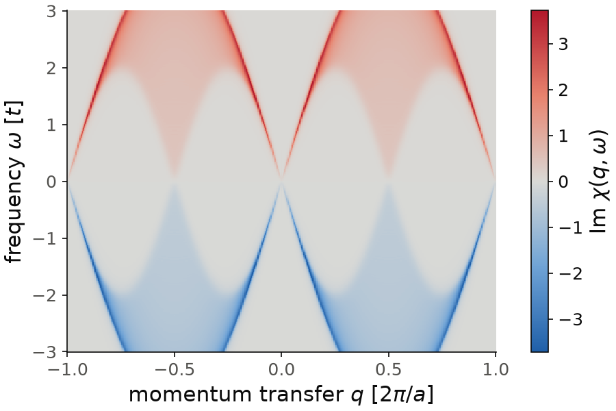
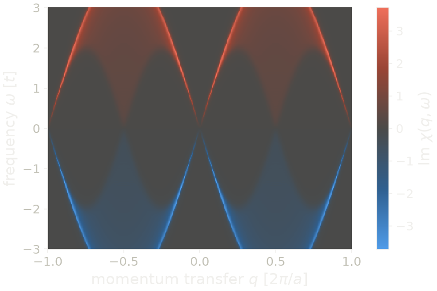
For the chain \(\epsilon_k=2t\cos k\), and at half filling the continuum at momentum transfer \(q\) goes from \(2t|\sin 2\pi q|\) up to \(4t|\sin\pi q|\). The weight is largest at the upper edge, the dark red lines. At small \(q\) the continuum is a narrow line, \(\omega\approx 4\pi t\,q\), set by the Fermi velocity. At \(q=1/2\) it goes from zero up to \(4t\), above the window of the plot, which stops at \(3t\). The sign follows the frequency: red for \(\omega>0\), blue for \(\omega<0\). The k-mesh is converged: with nk=801 instead of 401 the map changes by less than \(0.01\), for a maximum of \(3.7\). The width of the edges is the broadening delta=0.05. A k-mesh that is too coarse for this broadening gives horizontal stripes inside the continuum, so when you make delta smaller, make nk larger too. The map takes about 20 seconds.

Code of this figure (documentation/figures/charge_map.py)

import numpy as np
import style
from pyqula import geometry
g = geometry.chain()
h = g.get_hamiltonian()
qs = np.linspace(-1.,1.,401)
es = np.linspace(-3.,3.,301) # frequencies
chis = [h.get_chi(q=[q,0.,0.],energies=es,nk=401,delta=0.05)[1] for q in qs]
chis = np.array(chis) # shape (len(qs), len(es))

def draw(ax, c):
    m = np.abs(chis.imag).max()
    im = ax.pcolormesh(qs, es, chis.imag.T, cmap=c.diverging,
                       vmin=-m, vmax=m, shading="nearest", rasterized=True)
    style.colorbar(im, ax, r"Im $\chi(q,\omega)$")
    ax.set_xlabel(r"momentum transfer $q$ [$2\pi/a$]")
    ax.set_ylabel(r"frequency $\omega$ [$t$]")

style.save(draw, "charge_map")

See examples/1d/charge_response/main.py for a runnable script, and jupyter-notebooks/functionalities/response_functions/03_charge_response.ipynb for an executed notebook.

Response of any pair of operators

The same formula works for any two operators \(A\) and \(B\),

\[ \chi_{AB}(q,\omega) = \frac{1}{N_k}\sum_{\mathbf k,n,m} \left[f(\epsilon_{\mathbf k,n}) - f(\epsilon_{\mathbf k+q,m})\right] \frac{ \langle \Psi_{\mathbf k,n}|A|\Psi_{\mathbf k+q,m}\rangle \langle \Psi_{\mathbf k+q,m}|B|\Psi_{\mathbf k,n}\rangle } { \epsilon_{\mathbf k,n} - \epsilon_{\mathbf k+q,m} - \omega + i\delta } , \]

where the perturbation couples to \(B\) and we measure \(A\). Taking \(A=B=S_x\) gives the transverse spin susceptibility. We put the chain in a Zeeman field along \(z\), so that the spin and the charge responses are different:

from pyqula import geometry
import numpy as np
g = geometry.chain()
h = g.get_hamiltonian(has_spin=True)
h.add_zeeman([0.,0.,0.5]) # Zeeman field along z, splits the bands by 1.0
sx = h.get_operator("sx") # any of the operators from the "Operators" section
es = np.linspace(0.,2.,401)
(es,chi) = h.get_chi(A=sx,B=sx,q=[0.02,0.,0.],energies=es,nk=2001,delta=0.02)

By default \(A=B\) is the identity, which gives the charge response above. Any operator of the Operators page (spin, valley, sublattice, position, Nambu) can be used, which gives the corresponding susceptibility. Note that the operator "sx" is the Pauli matrix \(\sigma_x\), without the factor \(1/2\). The operator "sz" would not show anything new here: it does not flip the spin, so with the field along \(z\) its response is exactly the charge response.

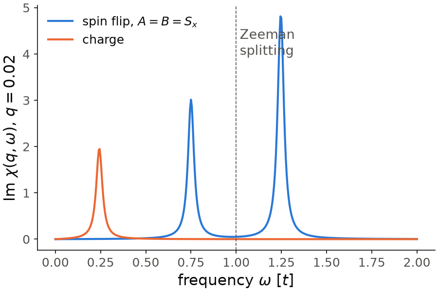
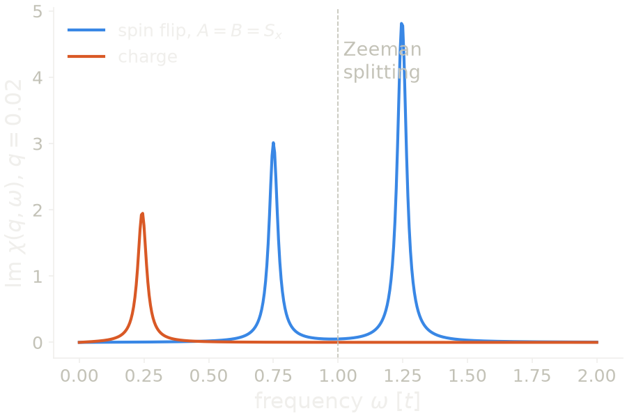
The field moves the two spin bands apart in energy by \(1.0t\), so flipping a spin costs the Zeeman splitting \(1.0t\). The charge response, in orange, does not flip the spin. An electron goes from \(k\) to \(k+q\) in the same band, which costs the Fermi velocity times \(q\), so there is one line at \(0.245t\). The spin response, in blue, has nothing there. A \(S_x\) perturbation moves an electron from one spin band to the other, so it costs the Zeeman splitting plus or minus the Fermi velocity times \(q\), and there are two lines, at \(0.75t\) and \(1.245t\), one for the electrons that move to the right and one for those that move to the left. At \(q=0\) the two lines merge into one at exactly \(1.0t\): this is the precession of the spins in the field, the line that electron spin resonance measures. The lines are sharp because at small \(q\) all the electron-hole pairs at this \(q\) have about the same energy. The k-mesh is converged: with nk=4001 the positions and the heights of the lines do not change. A finer delta makes the lines narrower and higher, and then nk has to grow with it.

Code of this figure (documentation/figures/charge_operator.py)

import style
from pyqula import geometry
import numpy as np
g = geometry.chain()
h = g.get_hamiltonian(has_spin=True)
h.add_zeeman([0.,0.,0.5]) # Zeeman field along z, splits the bands by 1.0
sx = h.get_operator("sx") # any of the operators from the "Operators" section
es = np.linspace(0.,2.,401)
(es,chi) = h.get_chi(A=sx,B=sx,q=[0.02,0.,0.],energies=es,nk=2001,delta=0.02)
(es,chic) = h.get_chi(q=[0.02,0.,0.],energies=es,nk=2001,delta=0.02) # charge, as a reference

def draw(ax, c):
    ax.plot(es, chi.imag, color=c.blue, label=r"spin flip, $A=B=S_x$")
    ax.plot(es, chic.imag, color=c.orange, label="charge")
    ax.axvline(1.0, color=c.ink2, lw=0.8, ls="--")
    ax.text(1.02, 0.95*chi.imag.max(), "Zeeman\nsplitting", color=c.ink2,
            va="top")
    ax.set_xlabel(r"frequency $\omega$ [$t$]")
    ax.set_ylabel(r"Im $\chi(q,\omega)$, $q=0.02$")
    ax.legend(loc="upper left")

style.save(draw, "charge_operator")

See jupyter-notebooks/functionalities/response_functions/04_operator_response.ipynb for an executed notebook.

RKKY interaction

Now we use the static response to couple two magnetic impurities. A magnetic moment in a metal polarizes the conduction electrons around it, and a second moment at some distance feels this polarization. The result is an effective exchange coupling between the two moments, the Ruderman-Kittel-Kasuya-Yosida (RKKY) interaction,

\[H_{\rm RKKY} = -J_{\rm RKKY}(\mathbf r)\, \vec S_i\cdot\vec S_j ,\]

where \(J_{\rm RKKY}(\mathbf r)\) is proportional to \(J_K^2\), with \(J_K\) the local exchange between each moment and the electrons, times the static spin response \(\chi_{ij}(\omega=0)\) of the electrons between the two sites at distance \(\mathbf r\). rkky.rkky_map computes it between a reference site and every other site up to some distance:

from pyqula import geometry
from pyqula import rkky
g = geometry.chain()
h = g.get_hamiltonian()
h.add_onsite(1.)
m = rkky.rkky_map(h,n=10,mode="LR",nk=200) # linear-response RKKY vs distance

The keywords are

• mode: "LR" computes the static response function above. "pm" puts a small magnetic field on each site and computes the change of the total energy, which is slower but needs no response function.
• n: up to how many unit cells away the coupling is computed.
• nk: number of k-points per direction for the sum over the Brillouin zone.

m has one row per site. The first three columns are the position \((x,y,z)\) of the site relative to the reference site, and the last column is the RKKY coupling:

x,e = m[:,0],m[:,3]

The coupling alternates in sign with the distance and decays, with a period \(\pi/k_F\) set by the Fermi wavevector \(k_F\). This is why the code moves the Fermi energy away from half filling with an onsite energy first. With the sign of \(H_{\rm RKKY}\) above, a positive value is a ferromagnetic coupling and a negative value an antiferromagnetic one. As a reference: for the chain at half filling, without the onsite energy, the coupling is negative (antiferromagnetic) at odd distances, between the two sublattices, and positive (ferromagnetic) at even distances, as expected for a bipartite lattice at half filling.

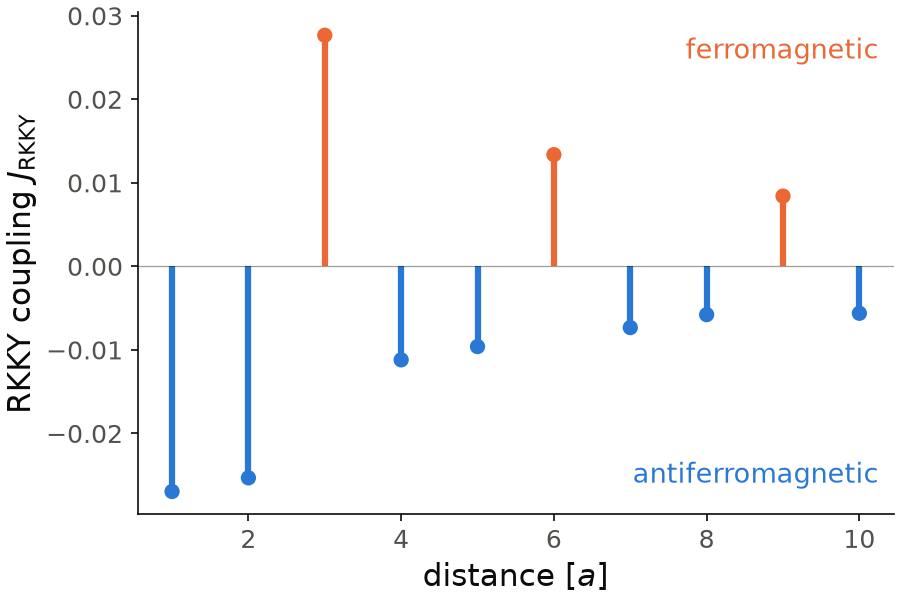
The onsite energy moves the band to \(2t\cos k+1\), so the Fermi energy is at \(\cos k_F=-1/2\), \(k_F=2\pi/3\), and the period \(\pi/k_F\) is \(1.5\) sites. On the lattice this gives a pattern that repeats every three sites: two antiferromagnetic values and one ferromagnetic value. The coupling is \(-0.027\), \(-0.025\) and \(+0.028\) at distances 1, 2 and 3, and it decays to \(-0.006\) at distance 10. Only the sites on one side are plotted, the other side is the same.

Code of this figure (documentation/figures/charge_rkky.py)

import numpy as np
import style
from pyqula import geometry
from pyqula import rkky
g = geometry.chain()
h = g.get_hamiltonian()
h.add_onsite(1.)
m = rkky.rkky_map(h,n=10,mode="LR",nk=200) # linear-response RKKY vs distance
x,e = m[:,0],m[:,3]
x,e = x[x>0],e[x>0] # keep one side, without the reference site

def draw(ax, c):
    col = [c.orange if v>0 else c.blue for v in e]
    ax.vlines(x, 0, e, color=col, lw=3)
    ax.scatter(x, e, color=col, s=40, zorder=3)
    ax.axhline(0, color=c.ink, lw=0.6, alpha=0.4)
    ax.set_xlabel("distance [$a$]")
    ax.set_ylabel(r"RKKY coupling $J_{\rm RKKY}$")
    ax.text(0.98, 0.95, "ferromagnetic", color=c.orange, ha="right",
            va="top", transform=ax.transAxes)
    ax.text(0.98, 0.05, "antiferromagnetic", color=c.blue, ha="right",
            va="bottom", transform=ax.transAxes)

style.save(draw, "charge_rkky")

See examples/1d/RKKY/main.py and examples/1d/rkky_minimal/main.py, which compares "pm" and "LR" on the same system, for runnable scripts, and jupyter-notebooks/functionalities/response_functions/05_rkky.ipynb for an executed notebook.