Excitons

When a semiconductor absorbs a photon, an electron goes to the conduction band and leaves a hole in the valence band. The electron and the hole attract each other, and they can form a bound state, the exciton. Its energy is below the band gap by the binding energy, so in an optical absorption measurement it is a peak below the absorption edge. A single-particle band structure cannot give this peak. We compute it here by solving the Bethe-Salpeter equation (BSE), the eigenvalue problem of an electron-hole pair, with h.get_bse() and h.get_exciton_energies().

Excitons and the Bethe-Salpeter equation

An exciton with center-of-mass momentum \(Q\) is a superposition of electron-hole pairs of the mean-field ground state \(|MF\rangle\),

\[|X\rangle_Q = \sum_{v,c,k} A_{vc}(k)\, c^\dagger_{c,k+Q}\, c_{v,k}\, |MF\rangle ,\]

where \(v\) runs over the valence bands, \(c\) over the conduction bands, and \(k\) over a k-mesh of \(N\) points. The amplitudes \(A_{vc}(k)\) are the wavefunction of the exciton in momentum space. They are the eigenvectors of the BSE Hamiltonian

\[H^{\rm BSE}_{vck,v'c'k'} = \left(\epsilon_{c,k+Q} - \epsilon_{v,k}\right)\delta_{vv'}\delta_{cc'}\delta_{kk'} + \frac{1}{N}\left(X_{vck,v'c'k'} - D_{vck,v'c'k'}\right).\]

The first term is the energy of a free electron-hole pair. The kernel has two terms. With \(C^{n,k}_a\) the coefficient of band \(n\) at \(k\) on orbital \(a\), the direct term is

\[D = \sum_{ab} C^{c,k+Q\,*}_a C^{c',k'+Q}_a\, W_{ab}(k-k')\, C^{v,k}_b C^{v',k'\,*}_b ,\]

the attraction between the electron and the hole through the interaction \(W\). It binds the exciton. The exchange term is

\[X = \sum_{ab} C^{c,k+Q\,*}_a C^{v,k}_a\, V_{ab}(Q)\, C^{c',k'+Q}_b C^{v',k'\,*}_b ,\]

the interaction between the charge densities of the two pairs. It is repulsive, it splits singlet and triplet excitons, and alone it gives the RPA. The orbitals are treated as point-like, as in the localized-orbital BSE of the Xatu code, arXiv:2307.01572. By default pyqula solves the full problem, which also couples the absorption pairs to the emission pairs (beyond the Tamm-Dancoff approximation).

By default the interaction is the one of a converged mean-field Hamiltonian, h.V. So the same interaction gives the Fock self-energy in h and the BSE kernel, and nothing is counted twice: this is time-dependent Hartree-Fock on top of Hartree-Fock. As an example, we converge a mean field on the gapped honeycomb lattice and compute its lowest excitons. Note that with these parameters the converged state is not magnetic: hmf.get_vev("sz") is of order \(10^{-5}\), so it is the band insulator of the sublattice imbalance. At this imbalance, \(0.6\), and with nk=6, the staggered moment appears only at about \(U=3.2\), where it is \(0.06\), and it is \(0.46\) at \(U=3.3\):

from pyqula import geometry
g = geometry.honeycomb_lattice()
h = g.get_hamiltonian(has_spin=True)
h.add_sublattice_imbalance(0.6)
hmf = h.get_mean_field_hamiltonian(U=1.5,filling=0.5,mf="antiferro",nk=6) # converge a mean field
es = hmf.get_exciton_energies(nk=6,n=8) # the eight lowest excitons

es contains the eight lowest exciton energies at \(Q=0\).

An onsite Hubbard \(U\) has a too short range to bind a Wannier-Mott exciton in two dimensions, so a realistic calculation needs a long-range interaction. bsetk.interaction.density_interaction builds a density-density interaction with the same parameters as the mean-field calculation (U, V1, V2, V3, or a function Vr of the two positions), and it is given to every exciton method with V=. Here it is a Coulomb tail \(V(r)=0.8/\sqrt{r^2+0.25}\) on a gapped honeycomb lattice:

import numpy as np
from pyqula.bsetk.interaction import density_interaction
h2 = g.get_hamiltonian()
h2.add_sublattice_imbalance(1.0) # a gapped semiconductor
W = density_interaction(h2,Vr=lambda r1,r2: 0.8/np.sqrt((r1-r2).dot(r1-r2)+0.25)) # Coulomb tail
bse = h2.get_bse(V=W,nk=21)
print(bse.get_energies()[0], bse.get_binding_energies()[0]) # lowest exciton, and how far below the gap

The binding energy is the lowest free electron-hole transition on the mesh minus the exciton energy, so a positive value means a bound exciton. With the Coulomb tail the lowest exciton separates from the band edge.

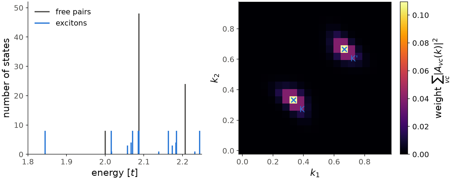
The figure is for the second snippet, with the Coulomb tail. On the left, each line is one energy and its height the number of states there. With nk=21 the mesh contains K and K', because 21 is a multiple of 3, so the lowest free pair is at the true gap \(2t\), with eight states: K and K', times four spin states. The next free pairs are at \(2.087t\) (48 states) and \(2.207t\) (24 states). The lowest exciton is at \(1.8445t\), so its binding energy is \(0.1555t\). It has eight states, two valleys times four spin states. The next excitons are at \(2.015t\) (eight states), \(2.016t\) (one state) and \(2.058t\) (three states), already above the gap. On the right is the weight \(\sum_{vc}|A_{vc}(k)|^2\) of the lowest exciton on the k-mesh, averaged over its eight states, with \(k_1,k_2\) in units of the reciprocal lattice vectors. The weight is a peak at K and K', where the gap is smallest, and it falls to almost zero within three or four points of the mesh. The binding energy is converged: it is \(0.1558t\) with nk=18, and the Large k-meshes section below finds \(0.1553t\) on meshes up to 30x30 in the Tamm-Dancoff approximation. A coarse mesh such as nk=8, which does not contain K, gives \(0.309t\), measured from its own band edge at \(2.165t\). The calculation takes about a minute.

Code of this figure (documentation/figures/excitons_bse.py)

import numpy as np
import style
from pyqula import geometry
from pyqula.bsetk.interaction import density_interaction
g = geometry.honeycomb_lattice()
h2 = g.get_hamiltonian()
h2.add_sublattice_imbalance(1.0) # a gapped semiconductor
W = density_interaction(h2,Vr=lambda r1,r2: 0.8/np.sqrt((r1-r2).dot(r1-r2)+0.25)) # Coulomb tail
bse = h2.get_bse(V=W,nk=21)
print(bse.get_energies()[0], bse.get_binding_energies()[0]) # lowest exciton, and how far below the gap

es = bse.get_energies() # all the exciton energies
de = bse.pairs.dE # energies of the free electron-hole pairs
lowest = np.isclose(es, es[0]) # the degenerate states of the lowest exciton
weight = np.zeros(len(bse.pairs.kpoints)) # |A(k)|^2 of the lowest exciton
for A in bse.amplitudes[lowest]:
    np.add.at(weight, bse.pairs.kindex, np.abs(A)**2)
weight = weight/np.sum(lowest) # average over the degenerate states
k1 = np.arange(21)/21 # the mesh, in units of the reciprocal lattice vectors

def draw(ax, c):
    for (e, color, label) in [(de, c.ink2, "free pairs"), (es, c.blue, "excitons")]:
        (levels, counts) = np.unique(e.round(4), return_counts=True)
        ax[0].vlines(levels, 0, counts, color=color, lw=2, label=label)
    ax[0].set_xlim(1.8, 2.25)
    ax[0].set_ylim(0, 52)
    ax[0].set_xlabel(r"energy [$t$]")
    ax[0].set_ylabel("number of states")
    ax[0].legend(loc="upper left")
    im = ax[1].pcolormesh(k1, k1, weight.reshape(21,21).T, cmap=c.cmap,
                          shading="nearest")
    style.colorbar(im, ax[1], r"weight $\sum_{vc}|A_{vc}(k)|^2$")
    ax[1].scatter([1/3, 2/3], [1/3, 2/3], marker="x", color=c.blue, s=60)
    ax[1].text(1/3+0.04, 1/3-0.04, "K", color=c.blue, va="top")
    ax[1].text(2/3+0.04, 2/3-0.04, "K'", color=c.blue, va="top")
    ax[1].set_aspect("equal")
    ax[1].set_xlabel("$k_1$")
    ax[1].set_ylabel("$k_2$")

style.save(draw, "excitons_bse", npanels=2)

• h.get_exciton_energies(): the exciton energies.
• h.get_exciton_binding_energies(): the binding energies (positive means bound).
• h.get_exciton_states(): the energies and the amplitudes \(A_{vc}(k)\).
• h.get_bse(): the solved problem; its pairs attribute gives the k-point and the two bands of each pair, to resolve the amplitudes in momentum or by band.
• Q=[qx,qy,qz]: excitons with finite center-of-mass momentum.
• nv, nc: keep only the nv highest valence and the nc lowest conduction bands.
• kernel: "full" (default) uses both terms; "direct" only the attraction, so no singlet-triplet splitting; "exchange" only the exchange, which is exactly the RPA; "none" no interaction, so the energies are the free transitions.
• tda=True: the Tamm-Dancoff approximation, which keeps only the absorption pairs. The matrix is four times smaller and Hermitian, and it is a good approximation at weak coupling.

The Hamiltonian is spinful, so the spin is part of the orbital index, and singlet and triplet excitons come from the same calculation. In a system with spin-rotation symmetry each free electron-hole transition is four times degenerate in spin. The full kernel can split it into a triplet, three times degenerate, and a singlet; neither of the two terms alone gives this 3+1 pattern. Not every level splits, and the singlet is not always the higher one. For the gapped honeycomb lattice with the Coulomb tail above, the lowest exciton stays eight times degenerate at \(1.8445t\), two valleys times four spin states. The 3+1 pattern appears higher up, with a singlet at \(2.016t\) below a triplet at \(2.058t\). With only an onsite term, density_interaction(h2,U=1.0) at nk=6, the singlet is above the triplet, at \(2.917t\) against \(2.704t\).

The default V=None reads h.V, which is only the \(z\) channel of an exchange interaction. It misses the \(x\) and \(y\) channels of an anisotropic exchange (J1x, J1y together with J1z), and it is zero after SxSx/SySy. In these cases build the interaction yourself and give it with V=.

The reference state must have a gap: a metal has no well-defined electron-hole pairs, and it is refused. Nambu (BdG) Hamiltonians are refused too. The problem has \(N_{\rm pair} = n_v n_c N\) pairs and a dense matrix of size \(2N_{\rm pair}\), so the k-mesh sets the cost. A calculation that needs more memory than max_memory (default 2 GB) is refused before it starts.

See jupyter-notebooks/functionalities/interacting_mean_field_hamiltonians/17_excitons_bse.ipynb for an executed notebook.

Large k-meshes

The k-mesh that an exciton needs depends on how strongly it is bound. A strongly bound exciton is small in real space, so it is spread over the Brillouin zone, and a coarse mesh is enough. A weakly bound Wannier-Mott exciton is large in real space, so its amplitude \(A(k)\) is a sharp peak at the band edge, and only a fine mesh resolves it. solver= chooses how to reach a fine mesh:

import numpy as np
from pyqula import geometry
from pyqula.bsetk.interaction import density_interaction
g = geometry.honeycomb_lattice()
h = g.get_hamiltonian()
h.add_sublattice_imbalance(1.0) # a gapped semiconductor
W = density_interaction(h,Vr=lambda r1,r2: 0.8/np.sqrt((r1-r2).dot(r1-r2)+0.25))
h.get_bse(V=W,nk=1024,tda=True,solver="iterative",neig=4)
h.get_bse(V=W,nk=65536,tda=True,solver="qtt",neig=1)

• solver="dense" (default): the whole exciton spectrum. The only one that works without the Tamm-Dancoff approximation. Good up to a few thousand pairs.
• solver="iterative": the same energies on much finer meshes, but only the neig lowest excitons.
• solver="qtt": for the very fine meshes of a weakly bound exciton. Only the lowest exciton.

"iterative" and "qtt" need tda=True, which is accurate for the weakly coupled systems where bound excitons appear. "qtt" works best on a fine mesh with few bands, which is the case of a Wannier-Mott exciton, and it is the best choice in 1D. In 2D use it on a primitive cell with small nv and nc; on a supercell, "iterative" is better. It needs nk to be a power of two, and it cannot take an RPA-screened interaction directly; give it one with ScreenedInteraction.get_dict().

See examples/1d/exciton_qtt/main.py and examples/2d/exciton_qtt/main.py for runnable comparisons of the three solvers, the second one plotting \(|A(k)|^2\) over the Brillouin zone, and examples/2d/excitons_bse/main.py for the lowest exciton of a gapped honeycomb lattice as the Coulomb tail grows. See jupyter-notebooks/functionalities/interacting_mean_field_hamiltonians/20_bse_matrix_free_qtt.ipynb for an executed notebook.

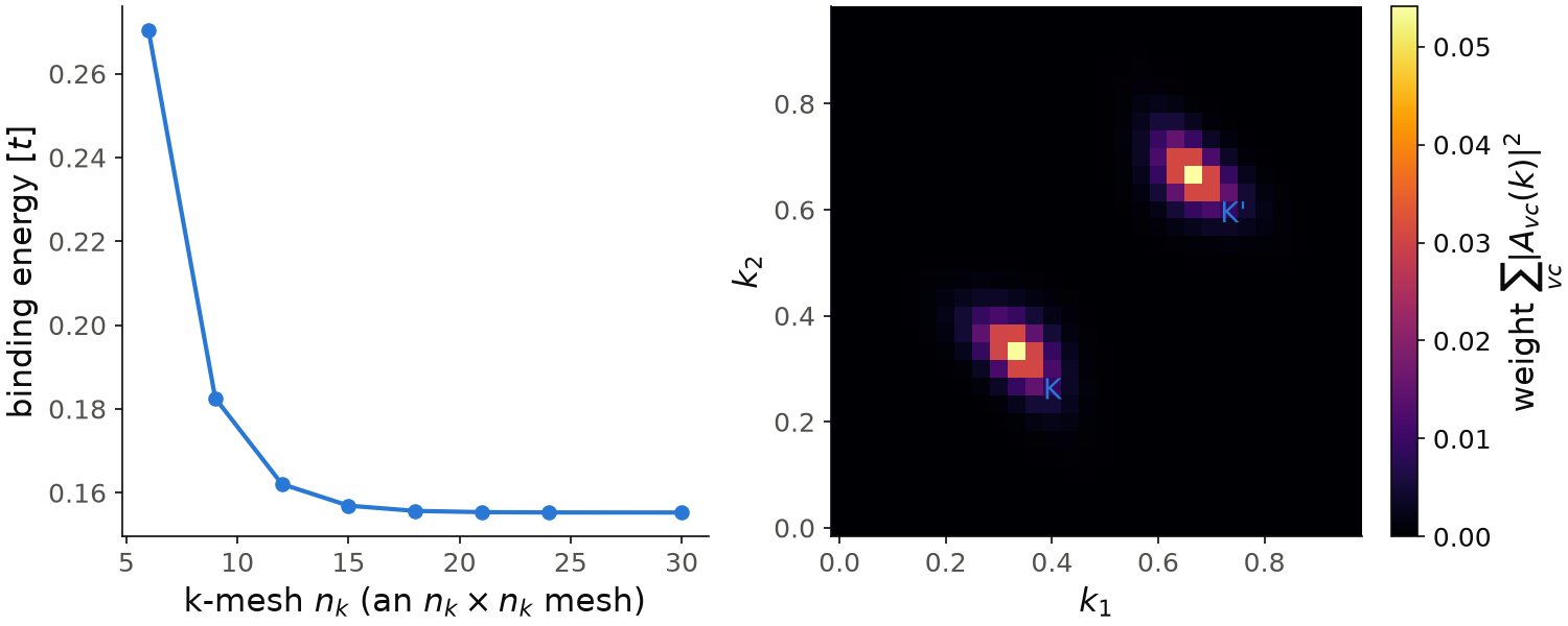
The figure uses the first solver of the snippet, solver="iterative", on meshes from 6x6 to 30x30 instead of nk=1024, so that it runs in about three minutes. Every mesh is a multiple of 3, so it contains K and K', the lowest free pair is at the true gap \(2t\), and the binding energy is measured from it. On the left, the binding energy is \(0.270t\) on the 6x6 mesh, \(0.162t\) on 12x12 and \(0.1553t\) on 30x30. From 21x21 on it changes by less than \(10^{-4}t\). On a coarse mesh the attraction is sampled on too few points, and the binding is overestimated. On the right is the weight \(\sum_{vc}|A_{vc}(k)|^2\) of the lowest exciton on the 30x30 mesh, averaged over the four states that the solver returns. It is a peak at K and K', the same in the two valleys, and it is close to zero at about \(0.15\) reciprocal lattice vectors from them, four or five points of the mesh. This exciton is strongly bound, so about 20x20 is enough. A weakly bound exciton has a narrower peak, and it needs the much finer meshes of the snippet.

Code of this figure (documentation/figures/excitons_largek.py)

import numpy as np
import style
from pyqula import geometry
from pyqula.bsetk.interaction import density_interaction
g = geometry.honeycomb_lattice()
h = g.get_hamiltonian()
h.add_sublattice_imbalance(1.0) # a gapped semiconductor
W = density_interaction(h,Vr=lambda r1,r2: 0.8/np.sqrt((r1-r2).dot(r1-r2)+0.25))
nks = [6,9,12,15,18,21,24,30] # meshes up to 30x30 instead of nk=1024
eb = [] # binding energy of the lowest exciton on each mesh
for nk in nks:
    bse = h.get_bse(V=W,nk=nk,tda=True,solver="iterative",neig=4)
    eb.append(bse.get_binding_energies()[0].real)
    print(nk, bse.get_energies()[0].real, eb[-1]) # lowest exciton, and how far below the gap

nk = nks[-1] # weight |A(k)|^2 of the lowest exciton on the finest mesh
weight = np.zeros(len(bse.pairs.kpoints))
for A in bse.amplitudes:
    np.add.at(weight, bse.pairs.kindex, np.abs(A)**2)
weight = weight/len(bse.amplitudes) # average over the four states
k1 = np.arange(nk)/nk # the mesh, in units of the reciprocal lattice vectors

def draw(ax, c):
    ax[0].plot(nks, eb, "o-", color=c.blue)
    ax[0].set_xlabel("k-mesh $n_k$ (an $n_k\\times n_k$ mesh)")
    ax[0].set_ylabel(r"binding energy [$t$]")
    im = ax[1].pcolormesh(k1, k1, weight.reshape(nk,nk).T, cmap=c.cmap,
                          shading="nearest")
    style.colorbar(im, ax[1], r"weight $\sum_{vc}|A_{vc}(k)|^2$")
    ax[1].text(1/3+0.05, 1/3-0.05, "K", color=c.blue, va="top")
    ax[1].text(2/3+0.05, 2/3-0.05, "K'", color=c.blue, va="top")
    ax[1].set_aspect("equal")
    ax[1].set_xlabel("$k_1$")
    ax[1].set_ylabel("$k_2$")

style.save(draw, "excitons_largek", npanels=2)

Exciton band structure

An exciton moves through the crystal with center-of-mass momentum \(Q\), so it has its own dispersion \(E_X(Q)\), the exciton band structure. It is not the difference of two band energies, because the electron-hole interaction changes it. Its curvature gives the effective mass of the exciton, and a flat exciton band means a strongly bound, compact exciton. h.get_exciton_bands() solves one BSE for each \(Q\) on a path, and returns the result in the same form as h.get_bands():

# h2 and W as in the section above
import numpy as np
from pyqula import geometry
from pyqula.bsetk.interaction import density_interaction
g = geometry.honeycomb_lattice()
h2 = g.get_hamiltonian()
h2.add_sublattice_imbalance(1.0) # a gapped semiconductor
W = density_interaction(h2,Vr=lambda r1,r2: 0.8/np.sqrt((r1-r2).dot(r1-r2)+0.25))
# nv=nc=2 keeps both members of each spin-degenerate pair
opts = dict(V=W,nq=20,nk=8,nv=2,nc=2,n=4)
qs,es = h2.get_exciton_bands(**opts) # the four lowest excitons along the path
qs0,es0 = h2.get_exciton_bands(kernel="none",**opts) # the bare continuum

qs is the index of the q-point along the path and es the exciton energy, both flat arrays for a scatter plot. n keeps the n lowest excitons at each q-point, and the other arguments go to h.get_bse(). qpath takes the same input as in h.get_bands(), and \(Q\) does not have to be on the k-mesh. The second call, with kernel="none", gives the bottom of the free electron-hole continuum. The exciton band runs below this continuum along the whole path, and the distance between them is the binding energy at each \(Q\). If the mean-field state is unstable at some \(Q\), es is complex there. Each q-point is one full BSE, so small nv, nc and tda=True make a long path affordable.

The window nv, nc must not cut a degenerate pair of bands in half. In a spinful Hamiltonian without spin-orbit coupling or magnetic order, every band is two times degenerate. With nv=1 the calculation keeps an arbitrary state of the pair, and the exciton energies become arbitrary too: in a time-reversal symmetric model \(E_X(Q)\) is then not even in \(Q\). pyqula gives a warning in this case. Use even nv and nc for a spin-degenerate Hamiltonian.

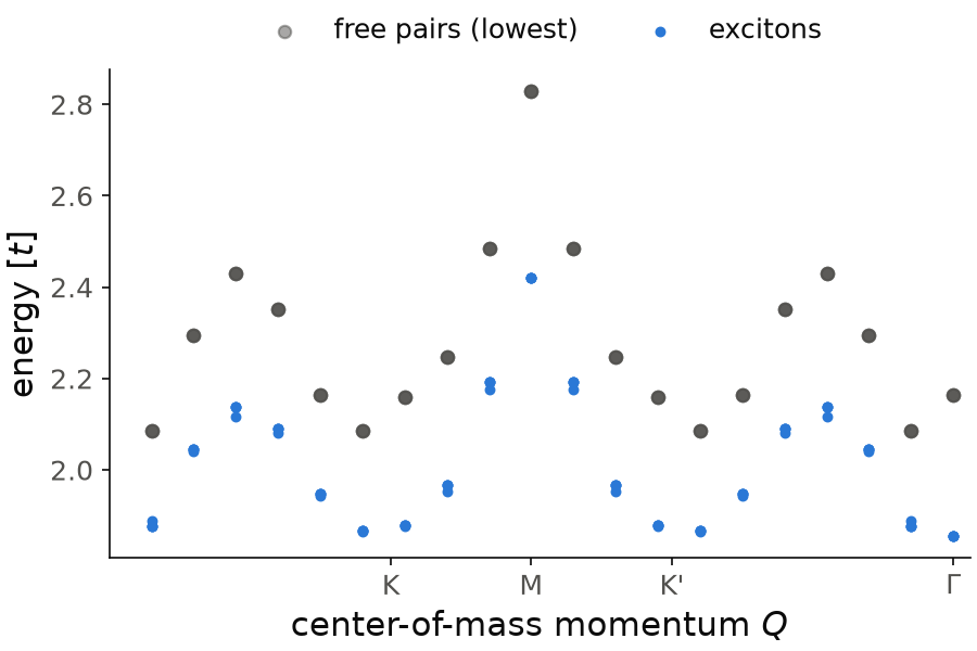
The default path goes from next to \(\Gamma\) through K, M and K' back to \(\Gamma\). The excitons (blue) are below the free pairs (gray) at every \(Q\). At \(\Gamma\) the lowest exciton is at \(1.856t\) and the lowest free pair at \(2.165t\); at M they are at \(2.42t\) and \(2.83t\). So the binding energy is between \(0.3t\) and \(0.4t\) along the whole path. Near K and K' the exciton band has a second minimum, \(1.864t\), almost as low as at \(\Gamma\): this is the exciton made of an electron in one valley and a hole in the other. Each blue point is close to a second one, the members of the spin multiplets.

Code of this figure (documentation/figures/excitons_bands.py)

# h2 and W as in the section above
import numpy as np
import style
from pyqula import geometry
from pyqula.bsetk.interaction import density_interaction
g = geometry.honeycomb_lattice()
h2 = g.get_hamiltonian()
h2.add_sublattice_imbalance(1.0) # a gapped semiconductor
W = density_interaction(h2,Vr=lambda r1,r2: 0.8/np.sqrt((r1-r2).dot(r1-r2)+0.25))
# nv=nc=2 keeps both members of each spin-degenerate pair
opts = dict(V=W,nq=20,nk=8,nv=2,nc=2,n=4)
qs,es = h2.get_exciton_bands(**opts) # the four lowest excitons along the path
qs0,es0 = h2.get_exciton_bands(kernel="none",**opts) # the bare continuum
x, x0 = (qs+1)/20, (qs0+1)/20 # position along the path, from Gamma through K, M, K to Gamma

def draw(ax, c):
    ax.scatter(x0, es0.real, s=30, color=c.ink2, alpha=0.5,
               label="free pairs (lowest)")
    ax.scatter(x, es.real, s=14, color=c.blue, label="excitons")
    ax.set_xticks([1/3, 1/2, 2/3, 1], ["K", "M", "K'", r"$\Gamma$"])
    ax.set_xlim(0, 1.02)
    ax.set_xlabel("center-of-mass momentum $Q$")
    ax.set_ylabel(r"energy [$t$]")
    ax.legend(loc="lower center", bbox_to_anchor=(0.5, 1.0), ncol=2)

style.save(draw, "excitons_bands")

See examples/2d/exciton_bands/main.py for a runnable script, with the exciton band of a gapped honeycomb lattice below its electron-hole continuum.

The screened interaction

So far the interaction in the kernel is the bare one. But an electron and a hole in a solid do not feel the bare interaction: the other electrons move around them and screen it. The mean-field calculation gives the bands \(\epsilon_{nk}\) and the coefficients \(C^{n,k}_a\) on a k-mesh, so the static RPA screening can be computed from them. The bare polarizability is

\[\chi^0_{ab}(q) = \frac{1}{N}\sum_k \sum_{n,m} (f_{nk}-f_{m,k+q})\, \frac{\rho^{nm}_a(k,q)\, \rho^{nm*}_b(k,q)}{\epsilon_{nk}-\epsilon_{m,k+q}}, \qquad \rho^{nm}_a(k,q) = C^{n,k*}_a C^{m,k+q}_a ,\]

where \(f\) is the occupation and \(a,b\) run over the spin-orbitals of the unit cell. The dielectric function and the screened interaction are

\[\varepsilon(q) = 1 - v(q)\chi^0(q), \qquad W(q) = \varepsilon^{-1}(q)\, v(q),\]

with \(v(q)\) the bare interaction. screening="rpa" puts \(W\) in the direct term:

import numpy as np
from pyqula import geometry
from pyqula.bsetk.interaction import density_interaction

h = geometry.honeycomb_lattice().get_hamiltonian()
h.add_sublattice_imbalance(1.0) # a gapped semiconductor

# a BARE interaction: an onsite term plus a soft-cutoff Coulomb tail
coulomb = lambda r1,r2: 0.6/np.sqrt((r1-r2).dot(r1-r2)+0.25)
V = density_interaction(h,U=1.0,Vr=coulomb)

bare = h.get_bse(V=V,nk=8) # time-dependent Hartree-Fock
screened = h.get_bse(V=V,nk=8,screening="rpa") # GW-BSE style

Compare the binding energies of bare and screened. With screening the binding is weaker, and the exciton is closer to the band edge, because the other electrons partly cancel the attraction between the electron and the hole.

The exchange term keeps the bare interaction for any screening. This is the usual GW-BSE choice: screening the exchange term too would count the same polarization bubbles twice. So kernel="exchange" does not change with screening, and pyqula gives a warning if both are set.

Do not screen a fitted Hubbard \(U\). A \(U\) chosen to describe a material is already a screened interaction, and screening it again makes it too weak. Screening is for a bare interaction: a Coulomb tail from density_interaction(Vr=...), or bare V1, V2, V3. The dangerous case is the default V=h.V of a Hubbard calculation.

screening="crpa" is the constrained RPA (arXiv:0710.4013): the transitions inside the nv, nc window are left out of the polarizability. Use it when the bands of the window are a downfolded model that will be solved exactly later. It screens less than the full RPA. It needs a real subset of the bands: with the default nv=nc=None the window is the whole spectrum, nothing is left to screen, and the call is refused.

The screened interaction is also available alone, as a ScreenedInteraction:

W = h.get_screened_interaction(V=V,nk=8)
print(W.epsmin) # smallest dielectric eigenvalue over the mesh
Wq = W.at(W.qs[3]) # the screened interaction at one q-point
d = W.get_dict() # ... and back in real space, usable at any q

\(W(q)\) exists only on the q-points of the mesh where it was computed, which are the ones the kernel needs; asking for another \(q\) raises an error. W.get_dict() gives \(W\) in real space, which can be evaluated at any \(q\), used to see how far the screened interaction reaches, or given to h.get_mean_field_hamiltonian(V=...) for a screened-exchange mean field. nkW sets a finer mesh for the screening than for the exciton, and must be an integer multiple of nk.

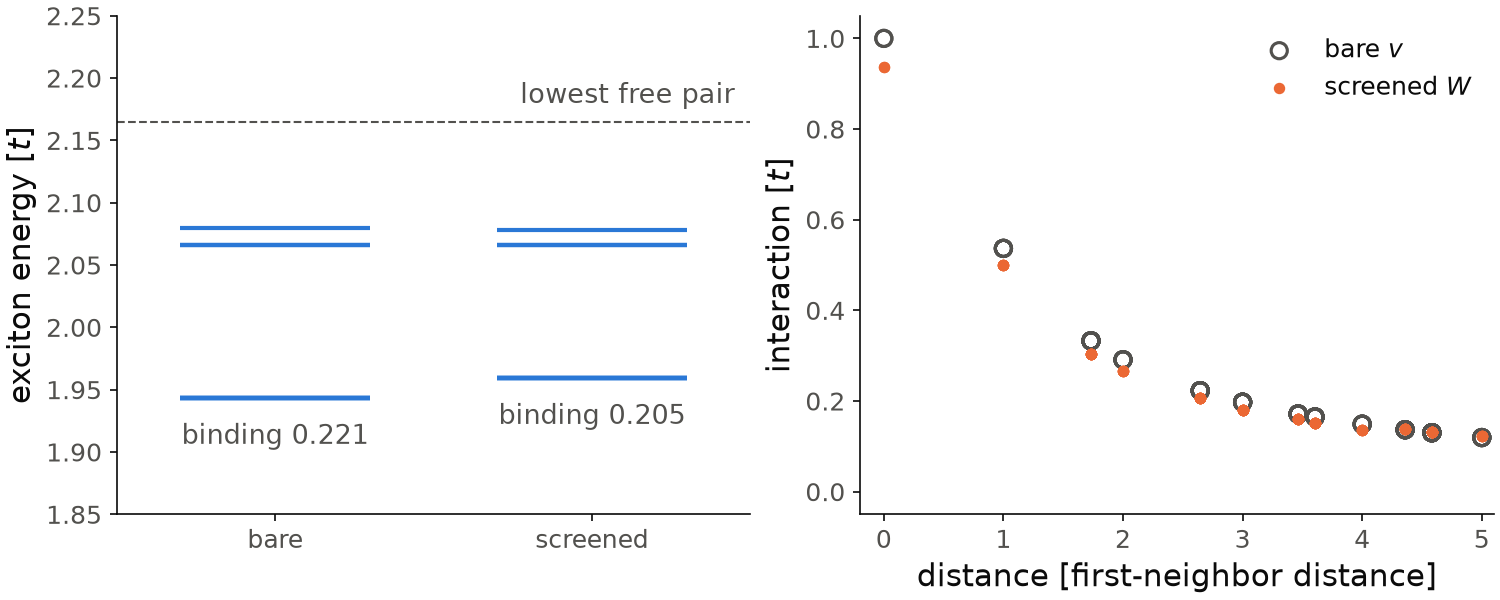
The figure uses the two snippets above. On the left, the lowest exciton moves up from \(1.943t\) to \(1.959t\) with screening, so the binding energy goes from \(0.221t\) to \(0.205t\). The higher excitons hardly move. On the right we take the interaction between opposite spins from V and from W.get_dict(), against the distance between the two sites; the first-neighbor distance is 1. The onsite term goes from \(1.0\) to \(0.94\), the first-neighbor term from \(0.537\) to \(0.50\), and the reduction becomes smaller at larger distance. So the screening is weak, a few percent, because the gap is large. W.epsmin is \(0.90\), below 1: along one direction the interaction becomes a little stronger, the case explained at the end of this section. The tail of V stops at distance 5, and \(W\) from an 8x8 mesh repeats every 8 unit cells, so we do not plot it further.

Code of this figure (documentation/figures/excitons_screening.py)

import numpy as np
import style
from pyqula import geometry
from pyqula.bsetk.interaction import density_interaction

h = geometry.honeycomb_lattice().get_hamiltonian()
h.add_sublattice_imbalance(1.0) # a gapped semiconductor

# a BARE interaction: an onsite term plus a soft-cutoff Coulomb tail
coulomb = lambda r1,r2: 0.6/np.sqrt((r1-r2).dot(r1-r2)+0.25)
V = density_interaction(h,U=1.0,Vr=coulomb)

bare = h.get_bse(V=V,nk=8) # time-dependent Hartree-Fock
screened = h.get_bse(V=V,nk=8,screening="rpa") # GW-BSE style

W = h.get_screened_interaction(V=V,nk=8)
print(W.epsmin) # smallest dielectric eigenvalue over the mesh
d = W.get_dict() # ... and back in real space, usable at any q

# the interaction between opposite spins on two sites, against their distance
r = h.geometry.r # positions of the two sites of the cell
a1, a2 = h.geometry.a1, h.geometry.a2
dist, v, w = [], [], []
for (n1,n2,n3) in V:
    for i in range(2):
        for j in range(2):
            dist.append(np.linalg.norm(r[j] + n1*a1 + n2*a2 - r[i]))
            v.append(V[(n1,n2,n3)][2*i,2*j+1].real) # spin up on i, down on j
            w.append(d[(n1,n2,n3)][2*i,2*j+1].real)

def draw(ax, c):
    for (x, b, label) in [(0, bare, "bare"), (1, screened, "screened")]:
        for e in b.get_energies()[:12]:
            ax[0].hlines(e, x-0.3, x+0.3, color=c.blue, lw=2)
        ax[0].text(x, b.get_energies()[0]-0.02, "binding %.3f" % b.get_binding_energies()[0],
                   color=c.ink2, ha="center", va="top")
    ax[0].axhline(bare.get_lowest_transition(), color=c.ink2, ls="--", lw=1)
    ax[0].text(1.45, bare.get_lowest_transition()+0.01, "lowest free pair",
               color=c.ink2, ha="right", va="bottom")
    ax[0].set_xticks([0, 1], ["bare", "screened"])
    ax[0].set_xlim(-0.5, 1.5)
    ax[0].set_ylim(1.85, 2.25)
    ax[0].set_ylabel(r"exciton energy [$t$]")
    ax[1].scatter(dist, v, s=60, facecolors="none", edgecolors=c.ink2,
                  lw=1.5, label="bare $v$")
    ax[1].scatter(dist, w, s=20, color=c.orange, label="screened $W$")
    ax[1].set_xlim(-0.2, 5.1)
    ax[1].set_xlabel("distance [first-neighbor distance]")
    ax[1].set_ylabel(r"interaction [$t$]")
    ax[1].legend(loc="upper right")

style.save(draw, "excitons_screening", npanels=2)

Screening acts on the charge. The total density polarizes the medium, and the induced charge acts back on the total density. So with channel="charge" (default) the dielectric matrix is built on the sites,

\[\varepsilon_{ij}(q) = \delta_{ij} - \sum_k v^c_{ik}(q)\,\chi^c_{kj}(q), \qquad \chi^c_{ij} = \sum_{\sigma\sigma'}\chi^0_{(i\sigma)(j\sigma')}, \qquad v^c_{ij} = \tfrac{1}{4}\sum_{\sigma\sigma'} v_{(i\sigma)(j\sigma')},\]

and the correction, which does not depend on spin, is added to the bare interaction,

\[W_{(i\sigma)(j\sigma')} = v_{(i\sigma)(j\sigma')} + \left[v^c \chi\, v^c\right]_{ij}, \qquad \chi = \chi^c(1-v^c\chi^c)^{-1}.\]

Note one convention: between two sites \(v^c_{ij}=V_{ij}\), but on the same site \(v^c_{ii}=U/2\) and not \(U\), because a Hubbard term couples only opposite spins, so only half of the density of a site acts on an electron there.

In the charge channel, spin-rotation symmetry is kept exactly. The other choice, channel="orbital", uses \(W=\varepsilon^{-1}v\) on the full spin-orbital matrix. It screens charge and spin with the same kernel, so it breaks spin-rotation symmetry, and an exciton multiplet that should be degenerate splits. Use the default. For a spinless Hamiltonian the two are the same.

Screening does not always make the interaction weaker. It does when the charge interaction \(v^c(q)\) is positive definite at every \(q\), as a physical repulsion is: the static charge response is negative, so \(\varepsilon = 1 - v^c\chi^c\) only reduces it. Without an onsite term, the interaction matrix has zero trace and has negative eigenvalues, and along them screening makes the interaction stronger. So include a realistic \(U\). \(U>0\) is not enough: the eigenvalues of \(v^c(q)\) are \(U/2\) plus those of the Fourier transform of the intersite interaction, which averages to zero over the Brillouin zone and so is negative somewhere. For example, on the square lattice a first-neighbor \(V_1\) gives \(U/2-4V_1\) at the corner of the zone, and \(U/2\) has to be larger than the most negative one.

If an eigenvalue of \(\varepsilon(q)\) reaches zero, the RPA diverges. This is a charge or spin instability of the mean-field state at this \(q\), the same condition \(1-V\chi=0\) that h.get_rpa_kernel_poles() gives as a collective mode (see Spin response and magnons), and the call raises an error.

• screening: the interaction of the direct term. None for the bare one, "rpa" for the screened \(W\), "crpa" for the constrained RPA.
• channel: where the dielectric matrix is built. Keep "charge", which keeps spin-rotation symmetry.
• nkW: the k-mesh of the screening, an integer multiple of nk. Increase it when the screening needs more k-points than the exciton.

See examples/2d/screened_bse/main.py for a runnable script, and jupyter-notebooks/functionalities/interacting_mean_field_hamiltonians/21_screened_interaction.ipynb for an executed notebook.