Topology in real space

A topological invariant is defined in the Brillouin zone, but its consequences are local: the bulk carries a quantized Berry flux and the edges carry the states that cross the gap. In this page we compute the Chern number from the local marker of a finite sample, also without any lattice, and the spectral function at the edge of a semi-infinite system.

Chern number in real space

The local marker \(C(\mathbf r)\) of Berry curvature density in real space is a number without units: the marker of a site divided by the area of the site. So in principle

\[ C = \frac{1}{A_{\rm cell}} \int_{\rm cell} C (\mathbf r)\, d^2 \mathbf r = \frac{\sum_{i} C_i A_i}{\sum_i A_i} , \]

the average of the marker over one unit cell of the bulk, with \(C_i\) the marker and \(A_i\) the area of the sites \(i\) of the cell. In a crystal every site of the cell has the same area, so this is the plain average over the sites of the cell, and every site of the bulk gives about \(C\). On a finite sample this has to be read with care. The sum of the marker, times the area of each site, over the whole island is exactly zero. So summing over all the sites does not give the invariant. What happens is the following. Deep inside a large enough island, the surroundings of a site look like the infinite bulk, and there the marker has a plateau at the bulk Chern number. The sites at the edge carry the opposite weight, which cancels it. This cancellation is the bulk-boundary correspondence in real space: the flux carried by the bulk is given back by the edge states.

from pyqula import islands
from pyqula import topology
import numpy as np
g = islands.get_geometry(name="honeycomb",n=8,nedges=3) # a honeycomb island
h = g.get_hamiltonian() # create hamiltonian of the system
h.add_haldane(0.05) # Add Haldane coupling
(r,c) = topology.real_space_chern(h) # local marker, per site
r = np.array(r)
bulk = np.argsort(np.linalg.norm(r-r.mean(axis=0),axis=1))[:len(r)//4] # innermost sites
C = np.mean(c[bulk]) # bulk plateau value approximates the total Chern number

The marker of each site is divided by the area of the site. This makes it a number without units, whose value in the bulk is the Chern number. The area of a site is the area of its Voronoi cell, the region of the plane closer to this site than to any other. In a crystal this is the area of the unit cell divided by the number of sites in it. The sites at the edge have open Voronoi cells, and they take the mean area of the others.

For this island the innermost quarter of the sites gives about \(1.95\), close to the \(C=2\) of the spinful Haldane model. The difference of a few percent comes from the small gap of \(t_2=0.05\). A small gap means a long decay length of the edge into the bulk, and the island with n=8 is not much larger than it, so its innermost quarter still feels the edge. A larger gap or a larger island removes the difference: with \(t_2=0.2\) the innermost sites give \(2.00\), and with \(t_2=0.05\) the islands with n=12 and n=16 give \(1.985\) and \(1.995\). The outermost sites are strongly negative, and the marker times the area adds up to zero over the whole island.

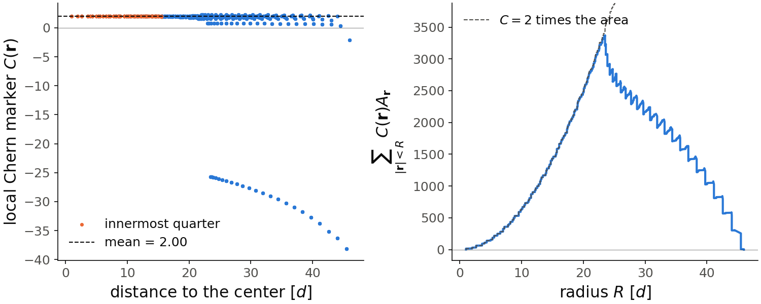
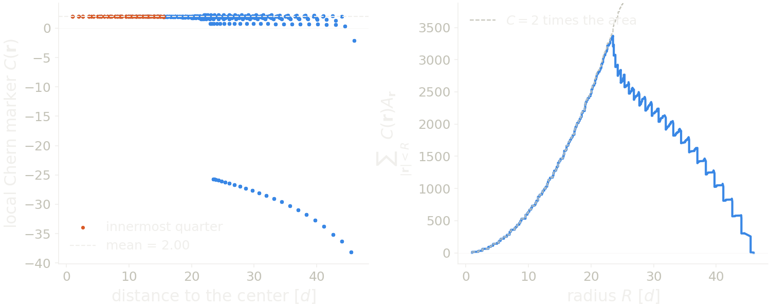
The figure uses the larger island, n=16, with 2301 sites, which takes about two minutes. On the left is the marker of each site against its distance to the center of the island. The innermost quarter of the sites, in orange, sits on the plateau, with mean \(1.995\). Further out the marker spreads, between about \(0.7\) and \(2.3\), and the sites at the edge go down to \(-38\). On the right we add up the marker times the area of each site, for the sites closer than \(R\) to the center. In the bulk every site gives about \(2\) times its area, so the sum follows \(2\) times the area inside \(R\) (dashed line). It grows up to \(R\approx23.5\), the distance from the center to the middle of an edge of the triangle, where it is \(3371\), against \(3440\) for \(2\) times the area. Then the edge sites come in, with their large negative marker, and the sum goes down to zero, within \(10^{-11}\), at the last site. This zero is exact for any finite island: the marker of a site is a diagonal element of the commutator of \(PxP\) and \(PyP\), with \(P\) the projector on the occupied states, and the sum of the diagonal elements, the trace, of a commutator of two finite matrices is zero. So the edge always gives back what the bulk carries.

Code of this figure (documentation/figures/realspace_marker.py)

import style
from pyqula import islands
from pyqula import topology
import numpy as np
from pyqula.topologytk.realspace import site_areas
g = islands.get_geometry(name="honeycomb",n=16,nedges=3) # a honeycomb island, larger than on the page
h = g.get_hamiltonian() # create hamiltonian of the system
h.add_haldane(0.05) # Add Haldane coupling
(r,c) = topology.real_space_chern(h) # local marker, per site
r = np.array(r)
bulk = np.argsort(np.linalg.norm(r-r.mean(axis=0),axis=1))[:len(r)//4] # innermost sites
C = np.mean(c[bulk]) # bulk plateau value approximates the total Chern number
d = np.linalg.norm(r-r.mean(axis=0),axis=1) # distance of each site to the center
A = site_areas(g) # area of each site
order = np.argsort(d) # sites from the center outwards
total = np.cumsum((c*A)[order]) # marker times area, summed up to a distance

def draw(axs, cl):
    ax = axs[0]
    ax.scatter(d, c, s=6, color=cl.blue)
    ax.scatter(d[bulk], c[bulk], s=6, color=cl.orange, label="innermost quarter")
    ax.axhline(C, color=cl.ink, lw=1, ls="--", label=f"mean = {C:.2f}")
    ax.axhline(0, color=cl.ink, lw=0.6, alpha=0.4)
    ax.set_xlabel("distance to the center [$d$]")
    ax.set_ylabel(r"local Chern marker $C(\mathbf{r})$")
    ax.legend(loc="lower left")
    axs[1].plot(d[order], total, color=cl.blue)
    axs[1].plot(d[order], 2*np.cumsum(A[order]), color=cl.ink2, lw=1, ls="--",
                label="$C=2$ times the area") # what a bulk of marker 2 would give
    axs[1].set_ylim(bottom=-0.05*total.max(), top=1.15*total.max())
    axs[1].legend(loc="upper left")
    axs[1].axhline(0, color=cl.ink, lw=0.6, alpha=0.4)
    axs[1].set_xlabel("radius $R$ [$d$]")
    axs[1].set_ylabel(r"$\sum_{|\mathbf{r}|<R}\, C(\mathbf{r})A_\mathbf{r}$")

style.save(draw, "realspace_marker", npanels=2)

An amorphous Chern insulator

The marker also works when there is no lattice at all. We take the amorphous Chern insulator of Agarwala and Shenoy. The sites are placed at random, uniformly and without correlations, in a square; this is what geometry.amorphous_lattice() builds. Each site has two orbitals. Every pair of sites closer than \(R=4\) is connected by a hopping that decays exponentially with the distance and depends on the direction of the bond. This dependence on the direction makes the model topological in a window of the mass \(M\).

from pyqula import geometry
from pyqula import topology
from pyqula.geometrytk import amorphous
from pyqula.topologytk.realspace import site_areas
import numpy as np
g = geometry.amorphous_lattice(L=36.,density=0.6,seed=0) # 778 sites at random positions
h = amorphous.amorphous_chern_hamiltonian(g,M=-0.5) # Agarwala-Shenoy model, half filling
(r,c) = topology.real_space_chern(h) # local marker, per site
A = site_areas(g) # area of the Voronoi cell of each site
bulk = np.max(np.abs(g.r[:,0:2]),axis=1)<6. # central square, far from the edges
C = np.sum(c[bulk]*A[bulk])/np.sum(A[bulk]) # area-weighted average of the marker

The two orbitals of each site play the role of the spin, so for pyqula h is spinful. The Hamiltonian is shifted so that the Fermi energy of half filling is at zero, which is where topology.real_space_chern() puts the Fermi energy. The marker now changes a lot from site to site, because no two sites have the same surroundings. And the sites do not have the same area, so the Chern number of a region is not the plain average of the marker, but its average weighted by the area of each site,

\[ C = \frac{\sum_{i} C_i A_i}{\sum_i A_i} . \]

This gives \(C\approx-1\). Agarwala and Shenoy find a Bott index of \(-1\) at this density in the window \(-2\lesssim M\lesssim1.2\), and the bulk marker goes to zero on both sides of it: sharply at \(M\approx-2\), and slowly at positive \(M\), where it is still about \(-1/2\) at \(M=1\), because the gap of a sample of this size closes slowly there.

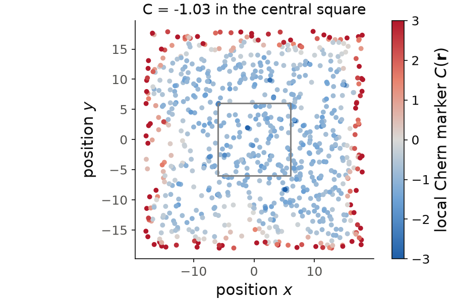
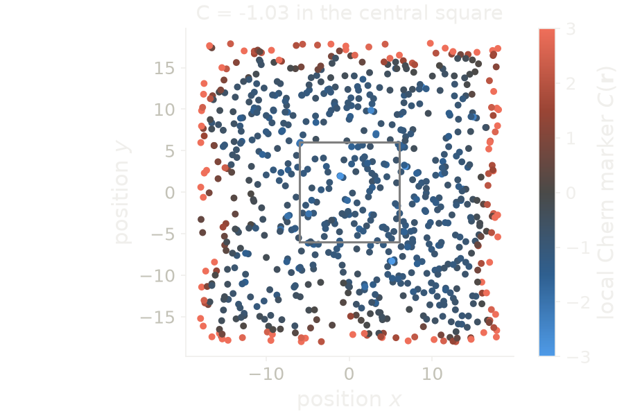
The figure shows the marker at each site of the snippet, with the central square of the average drawn in gray. Inside the sample the marker is negative at almost every site, around \(-1\), but it changes a lot from site to site. The area-weighted average over the central square is \(-1.03\). The sites at the edge of the sample are strongly positive, and they compensate the bulk, as on the island above.

Code of this figure (documentation/figures/realspace_amorphous.py)

import style
from pyqula import geometry
from pyqula import topology
from pyqula.geometrytk import amorphous
from pyqula.topologytk.realspace import site_areas
import numpy as np
g = geometry.amorphous_lattice(L=36.,density=0.6,seed=0) # 778 sites at random positions
h = amorphous.amorphous_chern_hamiltonian(g,M=-0.5) # Agarwala-Shenoy model, half filling
(r,c) = topology.real_space_chern(h) # local marker, per site
A = site_areas(g) # area of the Voronoi cell of each site
bulk = np.max(np.abs(g.r[:,0:2]),axis=1)<6. # central square, far from the edges
C = np.sum(c[bulk]*A[bulk])/np.sum(A[bulk]) # area-weighted average of the marker

def draw(ax, cl):
    sc = ax.scatter(g.r[:,0], g.r[:,1], c=c, s=14, cmap=cl.diverging, vmin=-3, vmax=3)
    style.colorbar(sc, ax, r"local Chern marker $C(\mathbf{r})$")
    ax.plot([-6,6,6,-6,-6], [-6,-6,6,6,-6], color="gray", lw=1.5) # the central square
    ax.set_aspect("equal")
    ax.set_xlabel("position $x$")
    ax.set_ylabel("position $y$")
    ax.set_title(f"C = {C:.2f} in the central square")

style.save(draw, "realspace_amorphous")

See jupyter-notebooks/functionalities/topological_characterization/05_real_space_chern_amorphous.ipynb for the maps of the Chern density and the two transitions.

Where local markers are useful

The real-space Berry curvature and the Chern marker are examples of a topological marker: a local quantity, computed from the ground-state projector only, that gives a bulk invariant without translational symmetry. So they are the tool for disordered systems, finite flakes, amorphous solids, or systems where the parameters change in space, for example a Haldane mass that changes sign across a boundary, or a topological insulator with dilute vacancies. The map of the marker shows where the invariant is carried, and where it changes.

Topological surface states

The invariant predicts states at the edge. The direct way to see them is the spectral function of a semi-infinite system: a half-plane, periodic along the edge and infinite away from it. The momentum along the edge is still a good quantum number, and the states localized at the edge appear as branches that cross the bulk gap. This is what ARPES sees on a surface, and what STM sees as in-gap density of states at an edge. For the Haldane model we use kdos.surface():

from pyqula import geometry
from pyqula import kdos
g = geometry.honeycomb_lattice() # create honeycomb lattice
h = g.get_hamiltonian() # create hamiltonian of the system
h.add_haldane(0.05) # Add Haldane coupling
kdos.surface(h) # surface spectral function

The call writes KDOS.OUT, with four columns: the momentum along the edge, the energy, the spectral weight at the surface and the spectral weight in the bulk. It also returns these four arrays, flat, with one entry per pair of momentum and energy. By default it uses a hundred energies between \(-1\) and \(1\) and a broadening delta=0.01. If you plot the surface weight as a function of momentum and energy, you see the chiral edge states crossing the gap, one for each unit of the Chern number. They are absent from the bulk weight: inside the gap the bulk weight is almost zero and the surface weight is not.

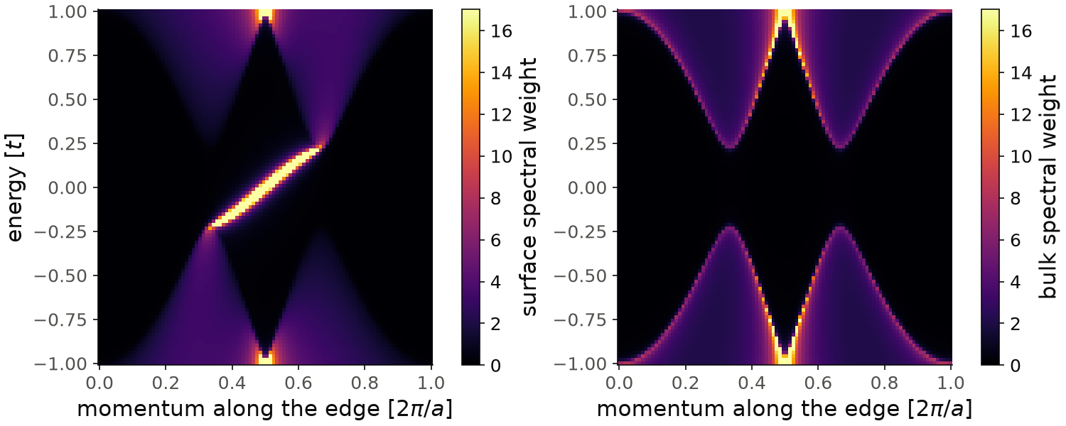
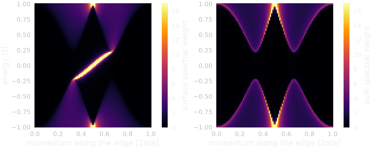
The figure shows the four arrays of the snippet, reshaped to \(100\) momenta times \(100\) energies: the surface weight on the left and the bulk weight on the right, with the same color scale, cut at the 99th percentile of the surface weight. The bulk weight shows the gap, from \(-0.225\) to \(0.225\), at the momenta \(1/3\) and \(2/3\), the projections of K and K'. In the surface weight one chiral branch crosses the gap, from \(-0.225\) at momentum \(1/3\) to \(0.225\) at momentum \(2/3\), through zero energy at momentum \(1/2\). The two spins give the same branch, on top of each other, so this one line carries the two units of \(C=2\).

Code of this figure (documentation/figures/realspace_surface.py)

import numpy as np
import style
from pyqula import geometry
from pyqula import kdos
g = geometry.honeycomb_lattice() # create honeycomb lattice
h = g.get_hamiltonian() # create hamiltonian of the system
h.add_haldane(0.05) # Add Haldane coupling
(k,e,ds,db) = kdos.surface(h) # surface spectral function
k,e = k.reshape(100,100),e.reshape(100,100) # 100 momenta times 100 energies
ds,db = ds.reshape(100,100),db.reshape(100,100) # surface and bulk weights

def draw(ax, c):
    for (axi,d,name) in zip(ax,[ds,db],["surface","bulk"]):
        im = axi.pcolormesh(k, e, d, cmap=c.cmap, vmin=0, vmax=np.percentile(ds,99))
        style.colorbar(im, axi, f"{name} spectral weight")
        axi.set_xlabel(r"momentum along the edge [$2\pi/a$]")
    ax[0].set_ylabel("energy [$t$]")

style.save(draw, "realspace_surface", npanels=2)

The same calculation is available as h.get_surface_kdos(), with the arguments energies, delta, kpath and operator, described in Spectral functions, together with the quantum spin Hall case. See examples/readme_examples/chern_surface_states/main.py and examples/2d/kdos_edge/main.py for scripts that make the plot.