Pseudofermion mean field

In this page we treat models of local spins with the same mean-field method as electrons. Each spin one half is written with an auxiliary fermion, the Abrikosov pseudofermion,

\[ \vec S_i=\tfrac12 \sum_{ss'} f^\dagger_{i,s}\vec\sigma_{ss'} f_{i,s'}, \qquad \sum_s f^\dagger_{i,s} f_{i,s}=1 , \]

with exactly one fermion on each site, because a spin one half has no charge fluctuations. You can think of the pseudofermion as the spin part of an electron, with the charge frozen. We use it first for the Heisenberg model, where it gives spinons, and then for the Kondo lattice, where it gives heavy fermions.

Spinon mean field for Heisenberg models

We take a spin-\(\tfrac12\) Heisenberg model,

\[ H=J\sum_{\langle ij\rangle}\vec S_i\cdot\vec S_j , \]

where no electron hops. With the pseudofermions, the exchange term is quartic in \(f\). Its mean-field decoupling gives a bond order parameter

\[ \chi_{ij}=\langle f^\dagger_i f_j\rangle , \]

which acts as a hopping for the pseudofermions, so they get a dispersion. These dispersing fermions are the spinons, and this is the resonating-valence-bond ansatz. The decoupling is the same one that the \(J\) channel of h.get_combined_mean_field_hamiltonian() does (see Exchange interactions), with two differences: the bare hopping is zero, and the constraint of one fermion is imposed on every site, not only on average. Each site gets its own Lagrange multiplier \(\lambda_i\), a local chemical potential, chosen so that \(\langle n_i\rangle = 1\). The construction follows section 4 of arXiv:1601.03742. SpinonHamiltonian (in pyqula.spinon) builds it:

from pyqula import geometry
from pyqula.spinon import SpinonHamiltonian

g = geometry.triangular_lattice() # a canonical frustrated-Heisenberg lattice
h = SpinonHamiltonian(g) # zero bare hopping, couplings come from J1/J2/...
h2 = h.get_mean_field_hamiltonian(J1=1.0,nk=12,mix=0.1,maxerror=1e-4)

h2.local_occupation   # <n_i> per site, exactly 1.0 at convergence
h2.constraint_lambda  # converged per-site Lagrange multiplier (local chemical potential)
h2.get_bands()        # spinon dispersion

The result is a spinon Hamiltonian:

• local_occupation: the occupation of each site, equal to one at convergence.
• constraint_lambda: the Lagrange multiplier \(\lambda_i\) of each site.
• h2.get_bands(): the spinon dispersion. In a quantum spin liquid these spin-\(\tfrac12\) excitations replace the magnons of an ordered magnet, and they appear as a continuum in inelastic neutron scattering.

The keyword filling is not accepted here, because the representation is only valid with exactly one fermion per site. Only the U(1) ansatz, with the bond order \(\chi_{ij}\) alone, is implemented. The Z2 ansatz, which also includes the pairing of spinons that \(J\) can induce, is not.

On a frustrated lattice (triangular, kagome) the converged state is not unique. Several self-consistent states, with different fluxes of \(\chi_{ij}\) around a plaquette, can exist at the same \(J\), and a random guess can land on any of them. This is part of the physics of the mean-field ansatz, not a problem of the loop. On a chain with one site per unit cell there is no frustration and the solution is unique, so repeated runs agree within maxerror. On a frustrated lattice, give an explicit mf to choose the ansatz you want.

A Zeeman field is already bilinear in \(f\), so it enters exactly, without any decoupling. We add it with h.add_zeeman() or h.add_exchange() on the SpinonHamiltonian, before the mean-field calculation:

h = SpinonHamiltonian(g)
h.add_zeeman([0., 0., 0.3])            # or h.add_exchange([0.,0.,0.3])
h2 = h.get_mean_field_hamiltonian(J1=1.0, nk=12)
h2.get_magnetization()                 # induced <sigma> per site, twice <S>

The vector \(\vec b\) given to h.add_zeeman() multiplies the Pauli matrices, not \(\vec S=\vec\sigma/2\). The term is \(+\vec b\cdot\vec\sigma=2\vec b\cdot\vec S_i\), so the induced \(\langle\vec S_i\rangle\) points opposite to \(\vec b\). This is the same convention as for electrons in Building a Hamiltonian. The constraint fixes the total occupation, not the spin, so it stays exact in a field, and \(\langle \vec S_i\rangle\) grows with the field until it saturates when the field is large compared with \(J\).

In a field the loop is fragile. With the snippet above, only 1 of 5 random seeds converges, and the converged state has a different bond order \(\chi_{ij}\) from the state without field, so its spinon band has another shape.

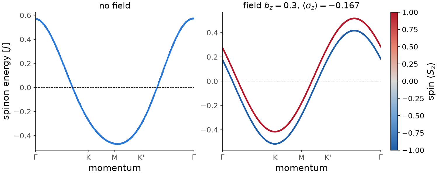
The script fixes the random seed, so that the figure is reproducible. On the left, the spinon band without field goes from \(-0.47\) to \(0.57\) in units of \(J\). It is half filled, so the spinons have a Fermi surface. On the right, with \(b_z=0.3\), the two spin bands are split by \(0.1\) and \(\langle\sigma_z\rangle=-1/6\), so \(\langle S_z\rangle=-1/12\) per site, against the field vector. The splitting is much smaller than the bare \(2b_z=0.6\). The reason is the exchange with the six neighbors, which adds a field \(6J\langle S_z\rangle=-0.5\) on \(S_z\) and cancels most of it. The band also changes its shape, because the bond order in the field is another one.

Code of this figure (documentation/figures/pseudofermions_spinon.py)

import numpy as np
import style
from pyqula import geometry
from pyqula.spinon import SpinonHamiltonian

np.random.seed(1) # fix the random guess, so that the figure is reproducible
g = geometry.triangular_lattice() # a canonical frustrated-Heisenberg lattice
h = SpinonHamiltonian(g) # zero bare hopping, couplings come from J1/J2/...
h2 = h.get_mean_field_hamiltonian(J1=1.0,nk=12,mix=0.1,maxerror=1e-4)
(k,e) = h2.get_bands() # spinon dispersion

h = SpinonHamiltonian(g)
h.add_zeeman([0., 0., 0.3])            # or h.add_exchange([0.,0.,0.3])
h2 = h.get_mean_field_hamiltonian(J1=1.0, nk=12)
(kb,eb,sz) = h2.get_bands(operator="sz") # spinon dispersion in the field, and Sz
m = h2.get_magnetization()             # induced <S> per site

def draw(axs, c):
    axs[0].scatter(k, e, s=3, color=c.blue)
    sc = axs[1].scatter(kb, eb, c=sz, s=3, cmap=c.diverging, vmin=-1, vmax=1)
    style.colorbar(sc, axs[1], r"spin $\langle S_z\rangle$")
    axs[0].set_title("no field")
    axs[1].set_title(r"field $b_z=0.3$, $\langle\sigma_z\rangle=%.3f$" % m[0][2])
    for ax in axs:
        n = k.max() # the path goes Gamma-K-M-K'-Gamma, K at one third
        ax.set_xticks([0, n/3, n/2, 2*n/3, n], [r"$\Gamma$", "K", "M", "K'", r"$\Gamma$"])
        ax.set_xlim(0, n)
        ax.axhline(0, color=c.ink, lw=0.8, ls="--") # Fermi level
        ax.set_xlabel("momentum")
    axs[0].set_ylabel("spinon energy [$J$]")

style.save(draw, "pseudofermions_spinon", npanels=2)
print(e.min(), e.max(), eb.min(), eb.max(), m)

See examples/spinon/heisenberg_chain/main.py and examples/spinon/heisenberg_chain_zeeman_field/main.py for runnable scripts, and the notebook jupyter-notebooks/functionalities/interacting_mean_field_hamiltonians/13_spinon_rvb.ipynb.

Kondo lattice

The Kondo lattice has a local moment on each site, coupled by exchange to a conduction electron on the same site. It is the minimal model of heavy-fermion compounds. We write it in the Coqblin-Schrieffer form of arXiv:cond-mat/0612006 (section II.C),

\[ H=\sum_k\epsilon_k c^\dagger_kc_k + \frac{J}{N}\sum_j \sum_{ab} S_{ab}(j)\,c^\dagger_{jb}c_{ja}, \qquad S_{ab}(j) = f^\dagger_{ja}f_{jb} - \frac{n_f}{N}\delta_{ab}, \]

with \(N=2\) for a spin one half, \(a,b\) the spin indices, and \(\epsilon_k\) the conduction band. Note that \(J\) here is the Coqblin-Schrieffer coupling, which enters as \(J/N\); it is not the coefficient of a Kondo term written as \(J\vec S_j\cdot\vec s_j\), and the two differ by a numerical factor. The moments are written with pseudofermions as before, and the exchange is decoupled into a hybridization field

\[ V_j=-\frac{J}{2}\sum_a\langle f^\dagger_{ja}c_{ja}\rangle , \]

together with a Lagrange multiplier \(\lambda_j\) that keeps one fermion per f-site. You can think of \(V_j\) as the amplitude for a conduction electron to turn into a spin flip of the local moment and back. This is the Read-Newns (large-\(N\)) mean field of the Kondo lattice.

KondoLatticeHamiltonian (in pyqula.kondolattice) takes a conduction-electron Hamiltonian and adds one localized f-site per conduction site, with zero bare hopping. Then it solves for \(V_j\) and \(\lambda_j\) self-consistently:

from pyqula import geometry
from pyqula.kondolattice import KondoLatticeHamiltonian

gc = geometry.chain()
hc = gc.get_hamiltonian(has_spin=True) # conduction electrons
h = KondoLatticeHamiltonian(hc)

seed = ([0.3+0.0j],[0.0]) # (V,lam), see the caveat below for why
h2 = h.get_mean_field_hamiltonian(J=1.5,filling=0.15,nk=200,mf=seed)

h2.local_occupation   # <n_f> per localized site, exactly 1.0 at convergence
h2.hybridization      # converged V per localized site
h2.constraint_lambda  # converged per-site Lagrange multiplier

The result is the heavy-fermion band structure. The conduction band hybridizes with a flat f-level at an energy set by \(\lambda_j\), and \(V_j\) opens a hybridization gap there. The bands on both sides of the gap are flat, heavy, because most of their weight is on the f-sites. This is the heavy-fermion band seen in ARPES, and the hybridization gap is seen in STM and optical spectroscopy. The three attributes are the occupation of each f-site, the hybridization \(V_j\) and the multiplier \(\lambda_j\).

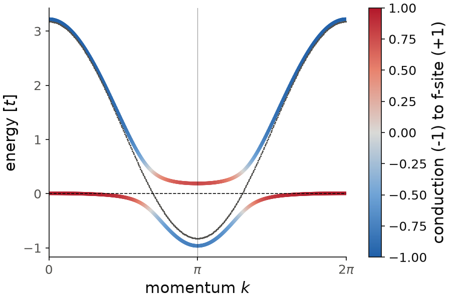
Energies are measured from the chemical potential (dashed line). Blue states live on the conduction sites and red ones on the f-sites. The gray line is the bare conduction band, \(2t\cos k\), as a reference. The f-level sits \(0.05\) above the chemical potential. The converged hybridization \(V_j=0.37\) mixes it with the conduction band, and a gap opens between the top of the lower band, at \(0.007\), and the bottom of the upper band, at \(0.19\). Close to the gap the bands are flat and mostly red: these are the heavy quasiparticles.

Code of this figure (documentation/figures/pseudofermions_kondo.py)

import numpy as np
import style
from pyqula import geometry
from pyqula.kondolattice import KondoLatticeHamiltonian

gc = geometry.chain()
hc = gc.get_hamiltonian(has_spin=True) # conduction electrons
h = KondoLatticeHamiltonian(hc)

seed = ([0.3+0.0j],[0.0]) # (V,lam), see the caveat below for why
h2 = h.get_mean_field_hamiltonian(J=1.5,filling=0.15,nk=200,mf=seed)
(k,e,f) = h2.get_bands(operator="zposition") # bands, and weight on the f-sites
k = 2*np.pi*k/k.max() # the k-path goes from 0 to 2 pi
(k0,e0) = hc.get_bands() # conduction band alone, as a reference
k0, e0 = 2*np.pi*k0/k0.max(), e0 - h2.fermi # energies from the chemical potential

def draw(ax, c):
    ax.plot(k0, e0, ".", ms=1, color=c.ink2)
    sc = ax.scatter(k, e, c=2*f-1, s=6, cmap=c.diverging, vmin=-1, vmax=1)
    style.colorbar(sc, ax, "conduction (-1) to f-site (+1)")
    ax.axhline(0, color=c.ink, lw=0.8, ls="--") # chemical potential
    style.kpath(ax, k, ["0", r"$\pi$", r"$2\pi$"])
    ax.set_xlabel("momentum $k$")
    ax.set_ylabel("energy [$t$]")

style.save(draw, "pseudofermions_kondo")

The keywords and caveats are:

• J: the Coqblin-Schrieffer coupling above.
• filling: sets the chemical potential once, from the bands with \(V=0\), and then keeps it fixed. The number of electrons can change while \(V\) and \(\lambda\) converge. The constraint \(\langle n_f\rangle=1\) is imposed by \(\lambda_j\), not by filling.
• mf: the initial \((V,\lambda)\). \(V=0\) is always a self-consistent solution, like the trivial solution of the BCS gap equation. A run without a seed starts there and stays there, even when a hybridized solution exists. So a nonzero seed, as above, is needed. When both exist, the hybridized state has the lower energy.
• T: the temperature of the Fermi-Dirac distribution, 0.02 by default.

Do not choose a filling that puts the chemical potential inside the flat f-level of the problem with \(V=0\). All the f-orbitals are then at the same energy \(\lambda\), and a wide range of fillings, roughly 0.25 to 0.75 for one conduction orbital per site, give the same ill-defined starting point. The filling=0.15 above keeps the chemical potential in the conduction band.

At zero temperature the large-\(N\) theory gives a hybridization for any \(J\), with a Kondo scale \(T_K=D\,e^{-1/(J\rho)}\), where \(D\) is the bandwidth and \(\rho\) the density of states. At the finite temperature T of the loop this becomes a crossover: below a threshold in \(J\), which depends on \(T\), \(V=0\) is the only solution, and at the threshold \(V\) jumps to a value of order one instead of growing continuously from zero.

A Zeeman field acts exactly on both the conduction electrons and the local moments, since both terms are bilinear. As for spinons, we add it with h.add_zeeman() or h.add_exchange() on the KondoLatticeHamiltonian, before the mean-field calculation:

h = KondoLatticeHamiltonian(hc)
h.add_zeeman([0., 0., 0.05])
h2 = h.get_mean_field_hamiltonian(J=1.5, filling=0.15, nk=150, mf=seed)

The field acts on every site, conduction and f. To put it on only one of the two, give a function of the position instead of a vector (the f-sites are shifted in \(z\)). The constraint \(\langle n_f\rangle=1\) stays exact in a field. The field competes with the Kondo singlet: at fixed \(J\), \(|V|\) decreases as the field grows, and a large enough field destroys the hybridized state. There the loop does not converge and the call raises an error, instead of giving a small nonzero \(V\). This is physics, not a numerical failure: it is the same decay to the \(V=0\) solution that a small \(J\) gives.

See examples/kondolattice/chain/main.py for a runnable script, and the notebook jupyter-notebooks/functionalities/interacting_mean_field_hamiltonians/14_kondo_lattice.ipynb.