Superconductivity

So far all our Hamiltonians contained only normal terms,

\[ H_0 = \sum_{ijss'} t_{ijss'}c^\dagger_{i,s} c_{j,s'} , \]

where \(i,j\) run over the sites and \(s,s'\) over the spin. Each term destroys one electron and creates one, so the number of electrons is conserved. In a superconductor there is also an anomalous term,

\[ H_{SC} = \sum_{ijss'} \Delta_{ij}^{ss'}c_{i,s} c_{j,s'} + h.c., \]

which destroys or creates a pair of electrons, so the number of electrons is not conserved anymore. The pairing amplitude \(\Delta_{ij}^{ss'}\) is the superconducting order parameter. In this page we add it by hand. In Mean-field Hubbard models we obtain it self-consistently from an attractive interaction.

The Nambu basis

To solve \(H = H_0 + H_{SC}\) we use the Nambu spinor of site \(n\),

\[ \Psi_n = \begin{pmatrix} c_{n,\uparrow} \\ c_{n,\downarrow} \\ c^\dagger_{n,\downarrow} \\ -c^\dagger_{n,\uparrow} \\ \end{pmatrix} . \]

You can think of it as the two electron operators of the site, stacked on top of their conjugates. In this basis a term that creates two electrons becomes a hopping between the upper and the lower half of the spinor, so the problem is again a single-particle one,

\[ H = \frac{1}{2}\Psi^\dagger \mathcal H \Psi + \text{const}, \]

where \(\mathcal H\) is the Bogoliubov-de Gennes (BdG) Hamiltonian, a matrix twice as large as the normal one. Its lower diagonal block is the hole copy of \(H_0\), and its off-diagonal blocks contain \(\Delta\). Diagonalizing it gives

\[ H = \sum_\alpha \epsilon_\alpha \gamma^\dagger_\alpha \gamma_\alpha + \text{const}, \]

with \(\gamma_\alpha\) the Bogoliubov quasiparticles. Because the lower half of the spinor is the conjugate of the upper half, the eigenvalues of \(\mathcal H\) come in pairs \(\pm\epsilon_\alpha\): every state has an electron copy and a hole copy. The gap of the spectrum around zero energy is \(2\min|\epsilon_\alpha|\).

h.setup_nambu_spinor() builds this doubled basis. h.add_swave() and h.add_pairing() build it themselves if it is not there. After this, every observable (band structure, density of states, LDOS) is computed in the Nambu basis. A Nambu Hamiltonian in pyqula is always spinful. For a superconducting mean-field calculation we call h.setup_nambu_spinor() before starting, as shown in Mean-field Hubbard models.

s-wave superconductivity

The simplest superconductor has spin-singlet s-wave pairing,

\[ H_{SC} = \Delta_0 \sum_n c_{n,\uparrow} c_{n,\downarrow} + h.c., \]

meaning that an electron with spin up and an electron with spin down on the same site form a pair, with the same amplitude \(\Delta_0\) on every site. This is the pairing of a conventional superconductor. We take a triangular lattice,

\[H = H_0 + H_{SC}, \qquad H_0 = \sum_{\langle ij\rangle} c^\dagger_i c_{j} + h.c.,\]

and add the pairing \(\Delta_0=0.2\) with h.add_swave():

from pyqula import geometry
g = geometry.triangular_lattice() # geometry of the 2D model
h = g.get_hamiltonian() # generate the Hamiltonian
h.add_swave(0.2) # add s-wave superconductivity
(k,e) = h.get_bands() # compute band structure

The BdG band structure shows both the electron and the hole bands. A gap opens at zero energy, from \(-\Delta_0\) to \(+\Delta_0\), so it is \(2\Delta_0\) wide. It opens at every point of the Fermi surface, whatever its momentum: this is the signature of s-wave pairing, and it is the hard gap that tunneling spectroscopy (STM) measures in a conventional superconductor. With operator="electron" in h.get_bands() each state is colored by its electron weight, so you can tell the electron copy from the hole copy, and read the electron spectral function, which is what ARPES measures.

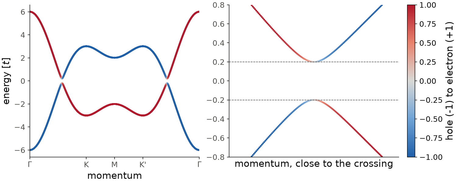
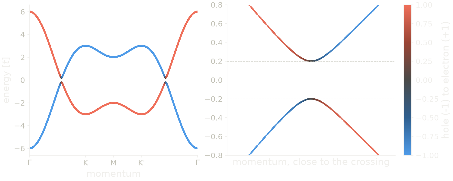
The figure uses nk=3000 points on the k-path, so that the zoom on the right is smooth. Red states are electrons and blue states are holes. The electron band goes from \(6\) at \(\Gamma\) to \(-3\) at K, and the hole band is its mirror image. Where the two bands cross zero energy they mix, the color goes to the middle of the scale, and a gap opens. The zoom on the right shows the gap edges at \(\pm0.2\) (dashed lines), so the gap is \(2\Delta_0=0.4\).

Code of this figure (documentation/figures/superconductivity_swave.py)

import style
from pyqula import geometry
g = geometry.triangular_lattice() # geometry of the 2D model
h = g.get_hamiltonian() # generate the Hamiltonian
h.add_swave(0.2) # add s-wave superconductivity
(k,e,c) = h.get_bands(operator="electron",nk=3000) # bands, and electron weight of each state

def draw(axs, col):
    n = k.max() # the path goes Gamma-K-M-K'-Gamma, K at one third
    for ax in axs:
        sc = ax.scatter(k, e, c=2*c-1, s=3, cmap=col.diverging, vmin=-1, vmax=1)
        ax.set_xticks([0, n/3, n/2, 2*n/3, n], [r"$\Gamma$", "K", "M", "K'", r"$\Gamma$"])
        ax.set_xlim(0, n)
        ax.set_xlabel("momentum")
    axs[0].set_ylabel("energy [$t$]")
    kf = k[k < n/3][abs(e[k < n/3]).argmin()] # where the bands cross zero
    axs[1].set_xlim(kf - n/40, kf + n/40) # zoom on the gap
    axs[1].set_ylim(-0.8, 0.8)
    axs[1].set_xticks([])
    axs[1].set_xlabel("momentum, close to the crossing")
    for y in [-0.2, 0.2]: axs[1].axhline(y, color=col.ink2, lw=0.8, ls="--")
    style.colorbar(sc, axs[1], "hole (-1) to electron (+1)")

style.save(draw, "superconductivity_swave", npanels=2)

The argument of h.add_swave() can also be a function of the position, to have a pairing that changes in space. For other pairing symmetries (p-wave, d-wave, a general d-vector) use h.add_pairing(delta=...,mode=...).

See examples/2d/comparison_swave/main.py for a runnable script, which adds the same gap with h.add_swave() and with h.add_pairing(mode="swave"). The notebooks jupyter-notebooks/functionalities/single_particle_hamiltonians/01_spinless_spinful_nambu_basis.ipynb and jupyter-notebooks/functionalities/single_particle_hamiltonians/03_magnetism_soc_superconductivity.ipynb show the Nambu basis, and superconductivity together with magnetism and spin-orbit coupling.

Spin-triplet pairing and the d-vector

In the s-wave case the two electrons of a pair form a spin singlet. The other possibility is a spin triplet, and we now see how to characterize it with h.get_dvector_non_unitarity(). For a triplet the pairing is a symmetric \(2\times2\) matrix in spin space, and we write it with a complex three-component vector \(\vec d\), the d-vector,

\[ \Delta = i (\vec d \cdot \vec \sigma) \sigma_y = \begin{pmatrix} -d_x + i d_y & d_z \\ d_z & d_x + i d_y \\ \end{pmatrix} . \]

So \(d_z\) is the opposite-spin pairing \(\Delta_{\uparrow\downarrow}\), and \(d_x,d_y\) give the equal-spin pairings \(\Delta_{\uparrow\uparrow}\) and \(\Delta_{\downarrow\downarrow}\). The component \(\Delta_{\uparrow\downarrow}\) can also contain a singlet part. The singlet is odd when we exchange the two spins and even when we exchange the two sites, the opposite of the triplet, and pyqula removes it before computing \(d_z\). So a state with both singlet and triplet pairing gives the d-vector of the triplet part only.

Triplet states are of two kinds. We compute

\[ \Delta \Delta^\dagger = |\vec d|^2 \mathbb{1} + \vec q \cdot \vec \sigma, \qquad \vec q = i (\vec d \times \vec d^*) . \]

• \(\vec q = 0\): the state is unitary. \(\Delta \Delta^\dagger\) is proportional to the identity, the two quasiparticle branches have the same gap, and the Cooper pairs have no net spin.
• \(\vec q \neq 0\): the state is non-unitary. The two spin branches have different gaps, and the pairs carry a spin moment \(\vec q\), which is a real vector.

If all the components of \(\vec d\) have the same phase, the state is always unitary. Non-unitarity needs a relative phase between the components, as in \(\vec d \propto (1, i, 0)\), which is pure \(\Delta_{\uparrow\uparrow}\) pairing with \(\vec q\) along \(+z\). So a non-unitary state breaks time-reversal symmetry. It appears naturally in ferromagnetic superconductors, where the pairs form in the majority band and \(\vec q\) is parallel to the magnetization.

h.get_dvector_non_unitarity() returns \(\vec q\) for each site, an array of shape (number of sites, 3). The d-vector is computed on a uniform k-mesh, \(\vec q\) is averaged over the mesh, and the contributions of all the pairing partners of a site are summed. As an example, we add by hand a p-wave pairing with \(\vec d \propto (1,i,0)\):

from pyqula import geometry
g = geometry.chain() # geometry of the 1D model
h = g.get_hamiltonian() # generate the Hamiltonian
h.setup_nambu_spinor() # initialize the Nambu basis
h.add_pairing(delta=0.3,mode="pwave",d=[1.,1j,0.]) # up-up pairing
q = h.get_dvector_non_unitarity(nk=20) # -> [[0., 0., 0.36]]

The array has one row, for the single site of the chain, and only its \(z\) component is not zero, because of the relative phase \(i\) between \(d_x\) and \(d_y\). The same p-wave pairing with a real d-vector, d=[1.,0.,0.], is unitary and gives zero.

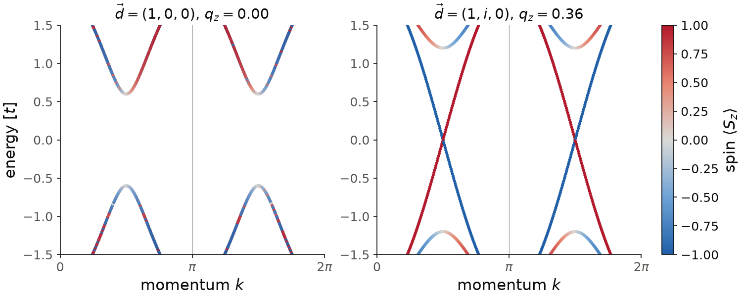
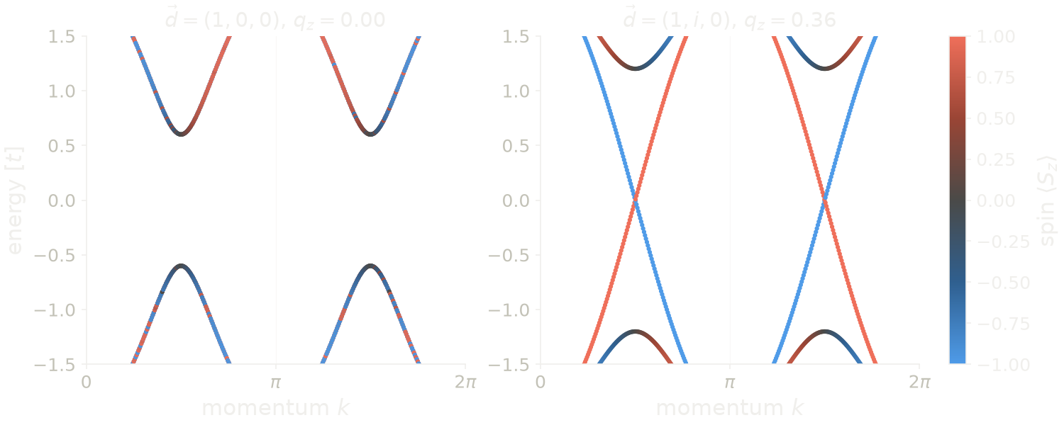
Here we compare the two d-vectors, with the same delta=0.3. With the real d-vector \((1,0,0)\), \(\vec q=0\) and both spins have the same gap, with edges at \(\pm0.6\). The two spin bands have the same energy, so the color of each state is a mix of the two. With \(\vec d=(1,i,0)\) only the spin-up electrons are paired. Their gap is twice as large, with edges at \(\pm1.2\), and the spin-down bands cross zero energy without any gap. These are the two different gaps of a non-unitary state.

Code of this figure (documentation/figures/superconductivity_dvector.py)

import style
from pyqula import geometry
g = geometry.chain() # geometry of the 1D model
h = g.get_hamiltonian() # generate the Hamiltonian
h.setup_nambu_spinor() # initialize the Nambu basis
h0 = h.copy() # keep the normal chain for the unitary state
h.add_pairing(delta=0.3,mode="pwave",d=[1.,1j,0.]) # up-up pairing
q = h.get_dvector_non_unitarity(nk=20) # -> [[0., 0., 0.36]]
h0.add_pairing(delta=0.3,mode="pwave",d=[1.,0.,0.]) # real d-vector, unitary
q0 = h0.get_dvector_non_unitarity(nk=20) # -> zero
bands = [h0.get_bands(operator="sz"), h.get_bands(operator="sz")] # (k,e,sz)
titles = [r"$\vec d=(1,0,0)$, $q_z=%.2f$" % q0[0][2],
          r"$\vec d=(1,i,0)$, $q_z=%.2f$" % q[0][2]]

def draw(axs, c):
    for (ax, (k,e,sz), t) in zip(axs, bands, titles):
        sc = ax.scatter(k, e, c=sz, s=4, cmap=c.diverging, vmin=-1, vmax=1)
        style.kpath(ax, k, ["0", r"$\pi$", r"$2\pi$"])
        ax.set_ylim(-1.5, 1.5)
        ax.set_xlabel("momentum $k$")
        ax.set_title(t)
    axs[0].set_ylabel("energy [$t$]")
    style.colorbar(sc, axs[1], r"spin $\langle S_z\rangle$")

style.save(draw, "superconductivity_dvector", npanels=2)

A non-unitary state can also come out of a self-consistent calculation. With an attractive first-neighbor interaction and a large exchange field (as in the long-range interaction example of Mean-field Hubbard models), the ground state is a spin triplet whose \(\vec q\) follows the magnetization:

from pyqula import geometry
g = geometry.triangular_lattice() # generate the geometry
h = g.get_hamiltonian() # create Hamiltonian of the system
h.add_exchange([0.,0.,3.]) # add exchange field
h.setup_nambu_spinor() # initialize the Nambu basis
# perform a superconducting non-collinear mean-field calculation
h = h.get_mean_field_hamiltonian(V1=-1.5,filling=0.3,mf="random",nk=30)
q = h.get_dvector_non_unitarity(nk=30) # antiparallel to +z, as is h.get_magnetization()

Other related methods:

• h.write_non_unitarity(): writes \(\vec q\) as a map in real space, for an inhomogeneous system, in NON_UNITARITY_MAP.OUT with columns \((x,y,z,q_x,q_y,q_z)\).
• h.get_average_dvector(): returns \((|d_x|^2,|d_y|^2,|d_z|^2)\) averaged over the Brillouin zone. With non_unitarity=True it returns the averaged squares of the components of \(\vec q\), which say if the state is non-unitary but not in which direction.

See examples/1d/dvector_map/main.py (a self-consistent triplet state on a spin spiral, with its map of non-unitarity) and examples/2d/SC_symmetry/main.py (a mixed singlet and triplet pairing separated into its two parts) for runnable scripts. The notebook jupyter-notebooks/functionalities/interacting_mean_field_hamiltonians/07_order_parameter_identification.ipynb shows how to identify a self-consistent order parameter, and jupyter-notebooks/functionalities/interacting_mean_field_hamiltonians/16_dvector_nonunitarity.ipynb the non-unitarity.

Superfluid weight and BKT temperature

A finite pairing amplitude alone does not make a superconductor. What carries a supercurrent is the stiffness of the state against a twist of the phase of the order parameter. We compute it with h.get_superfluid_weight(). This stiffness is the superfluid weight \(D_s\),

\[ D_s^{ab} = \frac{1}{V}\frac{\partial^2 \Omega}{\partial Q_a \partial Q_b}, \]

the second derivative of the grand potential \(\Omega\) with respect to the wavevector \(\mathbf Q\) of the phase twist, \(\Delta \to \Delta e^{i\mathbf Q\cdot\mathbf r}\), at fixed \(|\Delta|\), with \(V\) the volume (area in two dimensions). The superfluid weight is proportional to the inverse square of the London penetration depth, so it is what a measurement of the magnetic penetration depth or of the kinetic inductance gives. pyqula computes it with the general multiband BdG formula of Phys. Rev. B 95, 024515.

The superfluid weight has two parts:

• the conventional part, from the band velocities, the only one in a single-band model.
• the quantum-geometric part, from the interband matrix elements. For an isolated flat band it is the integral of the quantum metric (Nat. Commun. 6, 8944). A flat band has no velocity, so all its stiffness is geometric, and this is why a flat band can be superconducting at all.

This split is only defined for uniform onsite pairing and with time-reversal symmetry; otherwise asking for it raises a ValueError, and only the total is available. We compute both parts for a square lattice away from half filling:

from pyqula import geometry
g = geometry.square_lattice() # geometry of the 2D model
h = g.get_hamiltonian() # generate the Hamiltonian
h.add_onsite(-0.6) # move away from half filling
h.add_swave(0.3) # BdG Hamiltonian with an s-wave gap

D = h.get_superfluid_weight(nk=20) # Cartesian (dim,dim) tensor
out = h.get_superfluid_weight(nk=20,decompose=True)
print(out["total"],out["conventional"],out["geometric"])
print(h.get_bkt_temperature(nk=20)) # Nelson-Kosterlitz criterion

D is a \(2\times2\) Cartesian tensor. On the square lattice it is isotropic, about \(0.76\) on the diagonal. With decompose=True the result is a dictionary, and its "geometric" entry is zero here: a single band has no other band to couple to, so all its stiffness is conventional. The geometric part appears only in a multiband model, mostly for a flat band.

The phase twist uses the full bond vector \(\mathbf R + \mathbf r_j - \mathbf r_i\) between two orbitals, not only the lattice vector \(\mathbf R\). This matters when the unit cell has more than one orbital. With the lattice vector alone, \(D_s\) is anisotropic on the honeycomb lattice, which the \(C_3\) symmetry forbids, and it changes if we describe the same crystal with a supercell. With the full bond vector the result is isotropic and the same for any supercell. At fixed \(|\Delta|\) the superfluid weight depends on where the orbitals sit (Phys. Rev. B 106, 014518). gauge="lattice" uses the lattice vector only, which is the convention of Nat. Commun. 6, 8944; h.get_quantum_metric() has the same keyword with the same default (see Quantum geometry).

In two dimensions the superfluid weight gives the Berezinskii-Kosterlitz-Thouless (BKT) temperature, through the Nelson-Kosterlitz criterion

\[ T_{\rm BKT} = \frac{\pi}{8} D_s(T_{\rm BKT}) , \]

which h.get_bkt_temperature() solves self-consistently in \(T\). For the square lattice above it gives \(T_{\rm BKT}\approx0.15\), in units of the hopping. \(|\Delta|\) is kept fixed and does not decrease with temperature, so this is an upper bound.

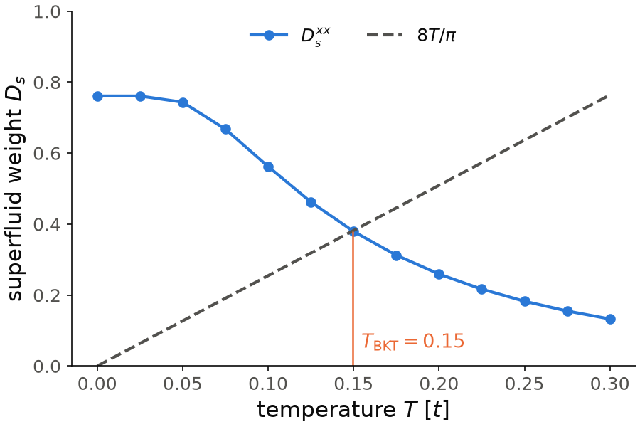
For this figure we compute \(D_s^{xx}\) at 13 temperatures with the keyword T, instead of the single call at \(T=0\). The superfluid weight is \(0.76\) at low temperature and stays flat up to \(T\approx0.05\). Then it decreases, because thermal quasiparticles reduce the stiffness. The BKT temperature is where the curve crosses the line \(8T/\pi\), at \(T=0.15\) with \(D_s=0.38\). Above it \(D_s\) does not go to zero, because \(|\Delta|\) is kept fixed.

Code of this figure (documentation/figures/superconductivity_superfluid.py)

import numpy as np
import style
from pyqula import geometry
g = geometry.square_lattice() # geometry of the 2D model
h = g.get_hamiltonian() # generate the Hamiltonian
h.add_onsite(-0.6) # move away from half filling
h.add_swave(0.3) # BdG Hamiltonian with an s-wave gap

Ts = np.linspace(0.,0.3,13) # temperatures, in units of the hopping
Ds = [h.get_superfluid_weight(nk=20,T=T)[0,0] for T in Ts] # D_s^xx at each T
Tbkt = h.get_bkt_temperature(nk=20) # Nelson-Kosterlitz criterion

def draw(ax, c):
    ax.plot(Ts, Ds, "o-", color=c.blue, label=r"$D_s^{xx}$")
    ax.plot(Ts, 8*Ts/np.pi, "--", color=c.ink2, label=r"$8T/\pi$")
    ax.vlines(Tbkt, 0, 8*Tbkt/np.pi, color=c.orange, lw=1.2)
    ax.text(Tbkt+0.005, 0.05, r"$T_{\rm BKT}=%.2f$" % Tbkt, color=c.orange)
    ax.set_xlabel("temperature $T$ [$t$]")
    ax.set_ylabel(r"superfluid weight $D_s$")
    ax.set_ylim(0, 1)
    ax.legend(loc="upper center", ncol=2)

style.save(draw, "superconductivity_superfluid")

Two keywords and one caveat:

• mode="finite_difference": computes the second derivative of \(\Omega\) numerically. It is much slower, but it does not use the assumptions of the analytic formula, so it is a good check.
• T: the temperature, in units of the hopping.

At \(T=0\), for a normal state without a gap and zero or very small pairing, the diamagnetic and paramagnetic parts should cancel. This cancellation comes from a term \(-\partial f/\partial E\) that becomes a delta function at \(T=0\), and a finite k-mesh cannot resolve it. So \(D_s\) comes out equal to the Drude weight of the normal state instead of zero. To check that a state has no stiffness, use a temperature that the k-mesh resolves.

See examples/2d/superfluid_weight/main.py for a runnable script, and jupyter-notebooks/functionalities/interacting_mean_field_hamiltonians/15_superfluid_weight.ipynb for an executed notebook.