Quantum transport

In this page we compute the conductance of junctions. We start with two normal leads, then a normal lead and a superconductor, and we end with the current through a junction between two superconductors at finite voltage.

A transport calculation has a scattering region between two semi-infinite leads. Each lead is a periodic Hamiltonian, of the kind built in Building a Hamiltonian. The leads enter through their self-energies \(\Sigma_L(E)\) and \(\Sigma_R(E)\), computed from the surface Green's function of each lead, and the Green's function of the scattering region is

\[G(E) = \left[E + i\delta - H_C - \Sigma_L(E) - \Sigma_R(E)\right]^{-1}.\]

For normal leads, the zero-temperature conductance is the Landauer formula,

\[G = \frac{e^2}{h}\, T(E), \qquad T(E) = {\rm Tr}\left[\Gamma_L\, G\, \Gamma_R\, G^\dagger\right], \qquad \Gamma_{L,R} = i\left(\Sigma_{L,R} - \Sigma_{L,R}^\dagger\right),\]

where \(T(E)\) is the transmission, the sum of the transmission probabilities of all the channels. pyqula gives conductances in units of \(e^2/h\), and counts the two spins as two channels, so a perfect spinful chain has \(G=2\). This is the differential conductance \(dI/dV\) at bias \(V=E/e\) that a two-terminal measurement gives.

When one lead is superconducting, the Hamiltonian is written in the Nambu basis (see Superconductivity), and the conductance is computed from the scattering matrix with the Blonder-Tinkham-Klapwijk formula,

\[G(E) = \frac{e^2}{h}\left[N - R_{ee}(E) + R_{he}(E)\right],\]

where \(N\) is the number of channels of the normal lead, \(R_{ee}={\rm Tr}\, r_{ee}^\dagger r_{ee}\) is the probability that an electron is reflected as an electron, and \(R_{he}={\rm Tr}\, r_{he}^\dagger r_{he}\) the probability that it is reflected as a hole. The second process is Andreev reflection: an electron from the normal side is reflected as a hole, and a Cooper pair enters the superconductor. It transfers a charge \(2e\), so it adds to the conductance.

Magnetoresistance in metal-metal transport

We now compute the conductance of a spin valve, a junction between two magnetic metals, with HT.didv(). We make two copies of the same chain and add an exchange field \(J\) to each of them. The first lead is magnetized along \(z\). In the second lead we rotate the magnetization in the \(xz\) plane, by an angle \(\theta\) from the first one, so \(\theta=0\) is the parallel and \(\theta=\pi\) the antiparallel configuration:

from pyqula import geometry
from pyqula import heterostructures
import numpy as np
g = geometry.chain() # create the geometry
h = g.get_hamiltonian() # create the Hamiltonian
h.add_onsite(1.0) # the band is now [-1,3], and E=0 is close to its bottom
thetas = np.linspace(0.,np.pi,61) # angles between the two magnetizations
def conductance(J,theta): # conductance at E=0 for exchange J and angle theta
    h1 = h.copy() ; h1.add_exchange([0.,0.,J]) # first lead, magnetization along z
    h2 = h.copy() ; h2.add_exchange([J*np.sin(theta),0.,J*np.cos(theta)]) # rotated in the xz plane
    HT = heterostructures.create_leads_and_central(h1,h2,h1) # create the junction
    return HT.didv(energy=0.0) # calculate conductance
Js = [0.3,0.6,0.9,1.5] # exchange strengths, the last one is a half metal
Gs = {J:np.array([conductance(J,t) for t in thetas]) for J in Js}

Gs[J] is the conductance \(G(\theta)\) at \(E=0\) for each angle, in units of \(e^2/h\). The onsite energy moves the Fermi energy close to the bottom of the band, so that a moderate exchange field changes the bands a lot. The exchange field splits the band into a majority band, \([-1-J,3-J]\), and a minority band, \([-1+J,3+J]\). For \(J<1\) both cross the Fermi energy, and the chain is a magnetic metal. For \(J>1\) the minority band is above the Fermi energy, and only one spin is a metal: this is a half metal.

In the parallel configuration each spin sees the same band on both sides, so it is transmitted perfectly. Then \(G(0)\) is 2 for \(J<1\), one per spin, and 1 for a half metal. When the second magnetization rotates, an electron in the majority band of the first lead has to enter the majority band of the second one, with its spin along the new direction. The overlap of the two spinors is \(\cos(\theta/2)\), so the transmission goes down with the angle. The magnetoresistance is

\[\mathrm{MR} = \frac{G_P - G_{AP}}{G_{AP}} ,\]

with \(G_P=G(0)\) and \(G_{AP}=G(\pi)\). This is what a spin valve measures: its resistance depends on the angle between the two magnetizations.

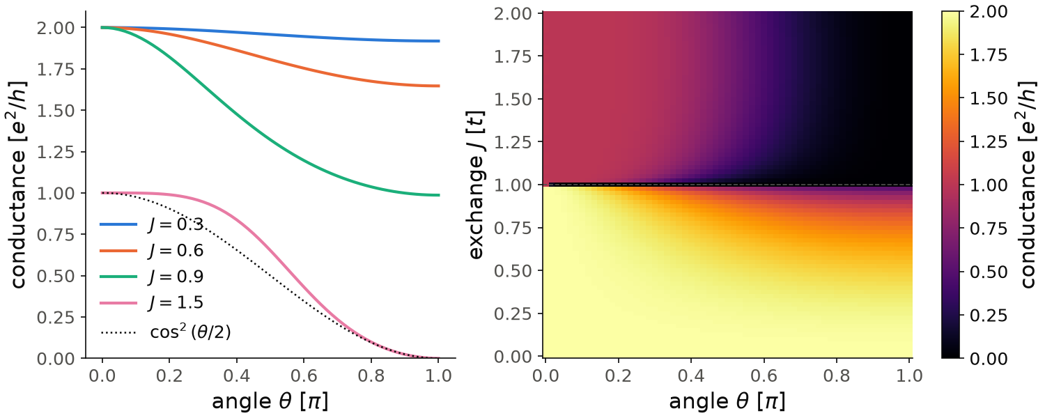
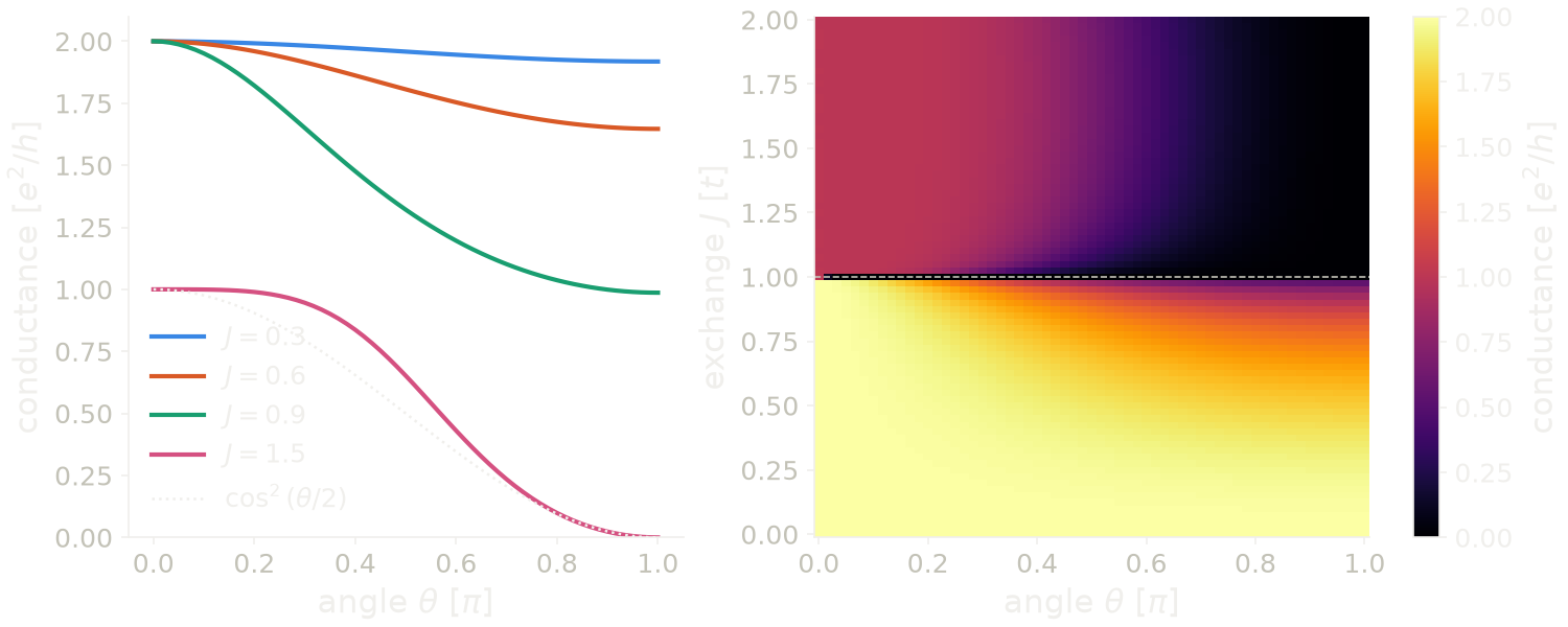
On the left, every curve starts at its parallel value and goes down smoothly to its minimum at \(\theta=\pi\). For \(J=0.3\) the antiparallel conductance is \(1.92\), so the magnetoresistance is only 4%, because the two spin bands are almost the same. It grows with the exchange field: \(G_{AP}\) is \(1.65\) for \(J=0.6\) and \(0.99\) for \(J=0.9\), where the minority band is close to leaving the Fermi energy, and the magnetoresistance is 103%. For the half metal, \(J=1.5\), the conductance goes from 1 at \(\theta=0\) to exactly zero at \(\theta=\pi\), so the magnetoresistance is infinite. An electron of the first lead has no state with its spin in the second lead, and the minority band of the second lead is above the Fermi energy. The curve is close to \(\cos^2(\theta/2)\) (dotted), the square of the overlap of the two spinors, but it is flatter near \(\theta=0\). The overlap alone is the answer of a tunnel contact, and this junction is a transparent one, so it does not have to follow it. The map on the right shows the conductance for all the exchange fields from 0 to 2. The dashed line, \(J=1\), separates the magnetic metal (below), where \(G(0)=2\), from the half metal (above), where \(G(0)=1\) and \(G(\pi)=0\).

Code of this figure (documentation/figures/transport_magnetoresistance.py)

import style
from pyqula import geometry
from pyqula import heterostructures
import numpy as np
g = geometry.chain() # create the geometry
h = g.get_hamiltonian() # create the Hamiltonian
h.add_onsite(1.0) # the band is now [-1,3], and E=0 is close to its bottom
thetas = np.linspace(0.,np.pi,61) # angles between the two magnetizations
def conductance(J,theta): # conductance at E=0 for exchange J and angle theta
    h1 = h.copy() ; h1.add_exchange([0.,0.,J]) # first lead, magnetization along z
    h2 = h.copy() ; h2.add_exchange([J*np.sin(theta),0.,J*np.cos(theta)]) # rotated in the xz plane
    HT = heterostructures.create_leads_and_central(h1,h2,h1) # create the junction
    return HT.didv(energy=0.0) # calculate conductance
Js = [0.3,0.6,0.9,1.5] # exchange strengths, the last one is a half metal
Gs = {J:np.array([conductance(J,t) for t in thetas]) for J in Js}
for J in Js: print("J =",J,"G_P =",Gs[J][0],"G_AP =",Gs[J][-1])

Jmap = np.linspace(0.,2.,81) # exchange strengths for the map
Gmap = np.array([[conductance(J,t) for t in thetas] for J in Jmap])

def draw(ax, c):
    for J,col in zip(Js, [c.blue, c.orange, c.green, c.magenta]):
        ax[0].plot(thetas/np.pi, Gs[J], color=col, label=f"$J={J:g}$")
    ax[0].plot(thetas/np.pi, np.cos(thetas/2)**2, ":", color=c.ink, lw=1.2,
               label=r"$\cos^2(\theta/2)$")
    ax[0].set_xlabel(r"angle $\theta$ [$\pi$]")
    ax[0].set_ylabel("conductance [$e^2/h$]")
    ax[0].set_ylim(0, 2.1)
    ax[0].legend(loc="lower left")
    im = ax[1].pcolormesh(thetas/np.pi, Jmap, Gmap, cmap=c.cmap, vmin=0, vmax=2,
                          shading="nearest")
    style.colorbar(im, ax[1], "conductance [$e^2/h$]")
    ax[1].axhline(1.0, color=c.ink2, lw=0.8, ls="--")
    ax[1].set_xlabel(r"angle $\theta$ [$\pi$]")
    ax[1].set_ylabel("exchange $J$ [$t$]")

style.save(draw, "transport_magnetoresistance", npanels=2)

See jupyter-notebooks/functionalities/quantum_transport/01_metal_metal_transport.ipynb for an executed notebook.

Superconductor-metal transport

We now compute the conductance between a normal metal and a superconductor, with heterostructures.build() and HT.set_coupling(). There are two limits. At a transparent contact, an electron with energy inside the gap cannot enter the superconductor as a quasiparticle, so it is Andreev reflected as a hole with probability one, and the conductance below the gap is twice the normal one. At a tunneling contact Andreev reflection is suppressed, because it needs two electrons to tunnel. Then the conductance follows the density of states of the superconductor: zero inside the gap, and coherence peaks at \(\pm\Delta\).

HT.set_coupling(T) multiplies the hopping between the two sides of the junction by \(T\), so \(T=1\) is a perfect contact and \(T\ll 1\) is a tunnel contact. The loop goes from one limit to the other:

from pyqula import geometry
from pyqula import heterostructures
import numpy as np
g = geometry.chain() # create the geometry
h = g.get_hamiltonian() # create the Hamiltonian
h1 = h.copy() # first lead
h2 = h.copy() # second lead
h2.add_swave(.01) # the second lead is superconducting
es = np.linspace(-.03,.03,100) # set of energies for dIdV
for T in np.linspace(1e-3,1.0,6): # loop over transparencies
    HT = heterostructures.build(h1,h2) # create the junction
    HT.set_coupling(T) # set the coupling between the leads
    Gs = [HT.didv(energy=e) for e in es] # calculate conductance

Gs is the conductance at each energy, for the last transparency of the loop. Compare it with its value outside the gap, \(|E|>\Delta=0.01\). At T=1.0 the conductance inside the gap is twice the one outside. At the smallest transparencies it goes to zero inside the gap and has peaks at the gap edges. This is the spectroscopy of a normal STM tip on a superconductor, and the transparency is what the experiment changes with the distance between the tip and the sample.

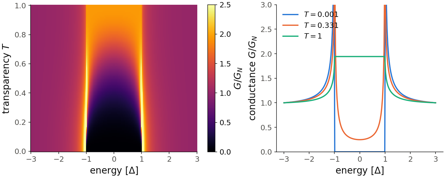
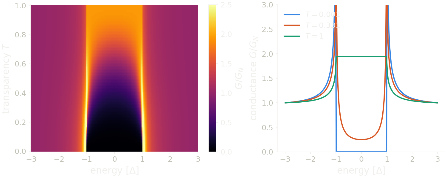
For the map we take 101 transparencies instead of 6, in steps of 0.01, and 201 energies, and we divide each curve by its value at \(E=-3\Delta\), outside the gap. With 16 transparencies the map had visible steps along \(T\). At \(T=1\) (top of the map, green curve) the conductance inside the gap is 1.94 times the one outside, close to the doubling of perfect Andreev reflection. When \(T\) goes down, the inside of the gap becomes dark: at \(T=0.331\) the conductance at \(E=0\) is 0.25, and at \(T=0.001\) it is \(2\times10^{-6}\). At the same time the coherence peaks at \(E=\pm\Delta\) appear, so the small-\(T\) curve (blue) is the BCS density of states. The color scale is cut at 2.5, so the peaks are saturated.

Code of this figure (documentation/figures/transport_andreev.py)

import style
from pyqula import geometry
from pyqula import heterostructures
import numpy as np
g = geometry.chain() # create the geometry
h = g.get_hamiltonian() # create the Hamiltonian
h1 = h.copy() # first lead
h2 = h.copy() # second lead
h2.add_swave(.01) # the second lead is superconducting
es = np.linspace(-.03,.03,201) # set of energies for dIdV
Ts = np.linspace(1e-3,1.0,101) # 101 transparencies instead of 6, for the map
Gmap = [] # conductance for each transparency
for T in Ts: # loop over transparencies
    HT = heterostructures.build(h1,h2) # create the junction
    HT.set_coupling(T) # set the coupling between the leads
    Gs = [HT.didv(energy=e) for e in es] # calculate conductance
    Gmap.append(np.array(Gs)/Gs[0]) # in units of the conductance outside the gap
Gmap = np.array(Gmap)
i0 = np.argmin(np.abs(es)) # E=0
for i in [0,20,33,50,80,100]: print("T =",Ts[i],"G(0)/G_N =",Gmap[i,i0],"max =",Gmap[i].max())

def draw(ax, c):
    im = ax[0].pcolormesh(es/0.01, Ts, Gmap, cmap=c.cmap, vmin=0, vmax=2.5,
                          shading="nearest")
    style.colorbar(im, ax[0], r"$G/G_N$")
    ax[0].set_xlabel(r"energy [$\Delta$]")
    ax[0].set_ylabel("transparency $T$")
    for i,col in zip([0,33,100], [c.blue, c.orange, c.green]):
        ax[1].plot(es/0.01, Gmap[i], color=col, label=f"$T={Ts[i]:.3g}$")
    ax[1].set_ylim(0, 3)
    ax[1].set_xlabel(r"energy [$\Delta$]")
    ax[1].set_ylabel(r"conductance $G/G_N$")
    ax[1].legend(loc="upper left")

style.save(draw, "transport_andreev", npanels=2)

See examples/transport/andreev_reflection/main.py for a runnable script, and jupyter-notebooks/functionalities/quantum_transport/02_metal_superconductor_transport.ipynb for an executed notebook.

Transport through an arbitrary finite region

In the two examples above, the scattering region is made of copies of the unit cell of the leads. We now use any finite (0d) Hamiltonian as the scattering region, for example a molecule or a quantum dot, with two semi-infinite chains attached at sites i and j, with h.get_central_heterostructure(i,j,left=None,right=None):

from pyqula import geometry

g = geometry.chain()
gc = g.get_supercell(5)
gc.dimensionality = 0 # a finite, 5-site cluster (no periodicity)
hc = gc.get_hamiltonian() # the central region, can be any 0d Hamiltonian

h_normal = g.get_hamiltonian() # normal lead
h_sc = g.get_hamiltonian(); h_sc.add_swave(0.05) # superconducting lead

ht = hc.get_central_heterostructure(0,4,left=h_normal,right=h_sc)
G = ht.didv(energy=0.02) # Andreev conductance, via the BdG scattering-matrix formula

G is the conductance at \(E=0.02\), inside the gap \(\Delta=0.05\) of the right lead, so it comes only from Andreev reflection. The result is a normal junction object, so didv, get_dos and get_kappa all work on it.

• left, right: the two leads. By default each is a spinless chain.
• j: the site of the second contact. By default the last site.
• At most one of hc, left and right can be superconducting. With two superconductors there is no normal lead to define the reflection, and the call raises a ValueError; use get_dc_current (below) instead.
• ht.landauer() only works for normal junctions, since the Landauer formula counts single electrons. With a superconductor use ht.didv().

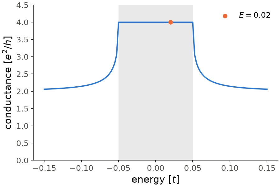
For the figure we compute the conductance on a grid of energies, besides the single value G at \(E=0.02\) (orange dot). Here the normal lead is spinful, so it has two channels, and the conductance far from the gap goes to 2. Inside the gap (shaded, \(|E|<0.05\)) it is 4.00, exactly two times 2: the cluster is a piece of the same chain, so nothing reflects the electrons at the contacts, and Andreev reflection is perfect. Just outside the gap the conductance decays slowly back to 2, it is still 2.06 at \(E=0.15\).

Code of this figure (documentation/figures/transport_central.py)

import numpy as np
import style
from pyqula import geometry

g = geometry.chain()
gc = g.get_supercell(5)
gc.dimensionality = 0 # a finite, 5-site cluster (no periodicity)
hc = gc.get_hamiltonian() # the central region, can be any 0d Hamiltonian

h_normal = g.get_hamiltonian() # normal lead
h_sc = g.get_hamiltonian(); h_sc.add_swave(0.05) # superconducting lead

ht = hc.get_central_heterostructure(0,4,left=h_normal,right=h_sc)
G = ht.didv(energy=0.02) # Andreev conductance, via the BdG scattering-matrix formula
es = np.linspace(-0.15,0.15,121) # energies across the gap, for the figure
Gs = [ht.didv(energy=e) for e in es]

def draw(ax, c):
    ax.axvspan(-0.05, 0.05, color=c.ink2, alpha=0.12, lw=0)
    ax.plot(es, Gs, color=c.blue)
    ax.scatter([0.02], [G], color=c.orange, zorder=3, label="$E=0.02$")
    ax.set_xlabel("energy [$t$]")
    ax.set_ylabel("conductance [$e^2/h$]")
    ax.set_ylim(0, 4.5)
    ax.legend(loc="upper right")

style.save(draw, "transport_central")

Only finite (0d) scattering regions are possible for now. See examples/transport/central_region_ij/main.py for a runnable script, and jupyter-notebooks/functionalities/quantum_transport/03_finite_central_region_two_leads.ipynb for an executed notebook.

Landauer transmission through a real-space device

There is a second way to build a junction, with multiterminal.Device. Here the leads and the scattering region are given as geometries, and the hoppings between them come from the real distances between the atoms. The transmission is the Landauer formula above, \(T_{ij}={\rm Tr}[\Gamma_i G \Gamma_j G^\dagger]\) between leads \(i\) and \(j\). This is useful for a disordered or irregular conductor, which has no unit cell to repeat.

import numpy as np
from pyqula import geometry
from pyqula import multiterminal

def lead_cell(x): # a one-site chain unit cell sitting at x
    g = geometry.chain() ; g.r = np.array([[x,0.,0.]]) ; g.r2xyz()
    return g

gc = geometry.chain().supercell(4) # the scattering region
xs = gc.r[:,0]
d = multiterminal.Device()
d.biterminal(left_g=lead_cell(min(xs)-1.),right_g=lead_cell(max(xs)+1.),
             central_g=gc,disorder=0.0)
print("ballistic transmission:",d.transmission(energy=0.0)[0])

A perfect chain has one open channel and nothing to scatter, so the transmission is 1 for every energy inside the band. With disorder larger than zero, random onsite energies are added in the scattering region, and the transmission goes below 1. Its value depends on the random configuration, so a disorder average needs several configurations. d.transmission(energy=e) returns a list with one value per pair of leads, by default only the pair (0,1). multiterminal.landauer(d,energy,ij=[(i,j)]) gives the same with the pairs written explicitly. The same disorder physics, with a chain of disordered cells between two clean leads, is in examples/transport/disordered_transport/main.py.

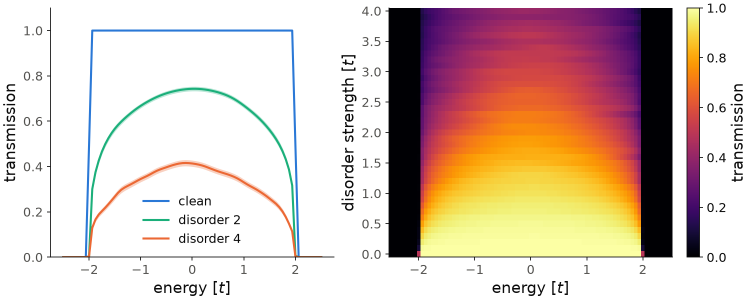
For the figure we compute the transmission at 81 energies, and we repeat it for 41 disorder strengths from 0 to 4, in steps of 0.1. Each point is the average over 400 random configurations, and the script takes about 17 minutes. The clean chain (blue) transmits 1 inside the band, \(|E|<2\), and 0 outside it; at the band edge \(E=\pm2\) it is 0.49. With disorder the transmission goes down, faster near the band edges than at the centre of the band. At \(E=0\) the average is \(0.74\) for a disorder 2 (green) and \(0.41\) for a disorder 4 (orange). The shaded bands are the statistical error of the average, the standard deviation over the configurations divided by \(\sqrt{400}\). It is at most \(0.015\), and it is what you still see as horizontal stripes in the map at strong disorder. With 100 configurations and another seed the error is twice as large, and the values at \(E=0\) are \(0.75\pm0.02\) and \(0.38\pm0.03\), the same within the error.

Code of this figure (documentation/figures/transport_device.py)

import numpy as np
import style
from pyqula import geometry
from pyqula import multiterminal
np.random.seed(1) # fixed seed, so that every run gives the same figure

def lead_cell(x): # a one-site chain unit cell sitting at x
    g = geometry.chain() ; g.r = np.array([[x,0.,0.]]) ; g.r2xyz()
    return g

gc = geometry.chain().supercell(4) # the scattering region
xs = gc.r[:,0]
d = multiterminal.Device()
d.biterminal(left_g=lead_cell(min(xs)-1.),right_g=lead_cell(max(xs)+1.),
             central_g=gc,disorder=0.0)
print("ballistic transmission:",d.transmission(energy=0.0)[0])

es = np.linspace(-2.5,2.5,81) # energies for the figure
Ws = np.linspace(0.,4.,41) # disorder strengths, in steps of 0.1
nconf = 400 # random configurations for each disorder strength
Tmap = np.zeros((len(Ws),len(es))) # transmission, averaged over disorder
Terr = np.zeros((len(Ws),len(es))) # statistical error of the average
for i,W in enumerate(Ws):
    Ts = []
    for n in range(nconf):
        d = multiterminal.Device()
        d.biterminal(left_g=lead_cell(min(xs)-1.),right_g=lead_cell(max(xs)+1.),
                     central_g=gc,disorder=W)
        Ts.append([d.transmission(energy=e)[0] for e in es])
    Tmap[i] = np.mean(Ts,axis=0)
    Terr[i] = np.std(Ts,axis=0)/np.sqrt(nconf)
i0 = np.argmin(np.abs(es)) # E=0
for i in [0,10,20,30,40]: print("W =",Ws[i],"T(E=0) =",Tmap[i,i0],"+-",Terr[i,i0])
print("largest statistical error:",Terr.max())

def draw(ax, c):
    ax[0].plot(es, Tmap[0], color=c.blue, label="clean")
    for i,col in [(20,c.green),(40,c.orange)]:
        ax[0].plot(es, Tmap[i], color=col, label=f"disorder {Ws[i]:g}")
        ax[0].fill_between(es, Tmap[i]-Terr[i], Tmap[i]+Terr[i], color=col, alpha=0.3, lw=0)
    ax[0].set_xlabel("energy [$t$]")
    ax[0].set_ylabel("transmission")
    ax[0].set_ylim(0, 1.1)
    ax[0].legend(loc="lower center")
    im = ax[1].pcolormesh(es, Ws, Tmap, cmap=c.cmap, vmin=0, vmax=1, shading="nearest")
    style.colorbar(im, ax[1], "transmission")
    ax[1].set_xlabel("energy [$t$]")
    ax[1].set_ylabel("disorder strength [$t$]")

style.save(draw, "transport_device", npanels=2)

Multiple Andreev reflection and AC-Josephson current

So far all the conductances are at zero temperature and in linear response. We now apply a finite voltage \(V\) to a junction between two superconductors, with HT.get_dc_current(). With a voltage, the phase difference of the two superconductors grows in time, \(\dot\phi = 2eV/\hbar\), so the problem is periodic in time with the Josephson frequency. Two things appear. The first is the AC Josephson effect. The second is multiple Andreev reflection (MAR): a quasiparticle is Andreev reflected many times between the two superconductors, and it gains an energy \(eV\) at each crossing, until it can leave above the gap. The process of order \(n\) opens when \(neV = 2\Delta\), so the current shows features at \(eV = 2\Delta/n\). What a measurement sees is the time-averaged current \(I_{dc}(V)\), and this is what is computed.

The voltage is moved by a gauge transformation into a time-dependent phase of the hopping between the two leads, \(t \to t\, e^{ieVt'/\hbar}\), and the problem is solved in Floquet space, with sidebands at energies \(\epsilon + n eV\). The DC current is

\[I_{dc}(V) = \frac{e}{h}\int_0^{eV} d\epsilon\; \sum_n {\rm Re}\,{\rm Tr}\left\{\left[G^r \Sigma_L^< + G^< \Sigma_L^a\right]_{nn} \tau_z\right\},\]

where \(G^r\) and \(G^<\) are the retarded and lesser Floquet Green's functions, \(\Sigma_L^<\) and \(\Sigma_L^a\) the lesser and advanced self-energies of the left lead, and \(\tau_z\) is \(+1\) for electrons and \(-1\) for holes. This is the formalism of San-Jose, Cayao, Prada and Aguado, arXiv:1301.4408. The current is in units of \(e/h\) times energy (in units of \(t\)), so that for two normal leads \(dI_{dc}/dV\) is the conductance in units of \(e^2/h\). It works for any pair of normal and superconducting leads, also for two superconductors, where the scattering formula of didv above cannot be used.

from pyqula import geometry
from pyqula import heterostructures
import numpy as np
g = geometry.chain() # create the geometry
h = g.get_hamiltonian() # create the Hamiltonian
h1 = h.copy() ; h1.add_swave(0.1) # left superconducting lead
h2 = h.copy() ; h2.add_swave(0.1) # right superconducting lead
HT = heterostructures.build(h1,h2) # junction between the two superconductors
HT.set_coupling(0.5) # set the normal transparency of the weak link
vs = np.linspace(0.02,1.5,40)*0.1 # bias voltages
Is = HT.get_iv_curve(vs) # MAR/AC-Josephson dc current

Is is the DC current at each voltage in vs, from \(0.02\Delta\) to \(1.5\Delta\), so all the voltages are below \(2\Delta=0.2\). There the current is carried by multiple Andreev reflections, and it shows steps at \(eV = 2\Delta/n\), sharper for a small transparency; the steps \(n=2,3,4\) are inside the window. Above \(2\Delta\), outside this window, the current grows roughly linearly with the voltage, as in a normal junction.

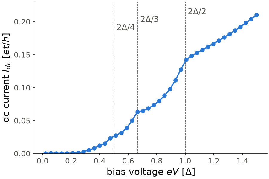
The figure is the snippet, with its 40 voltages from \(0.02\Delta\) to \(1.5\Delta\), and it runs in about two minutes. Below \(0.2\Delta\) the current is smaller than \(10^{-3}\). Then it grows in steps. It rises fast just below each voltage \(2\Delta/n\) and becomes flatter just above it. Across \(2\Delta/3\) it goes from \(0.050\) at \(0.63\Delta\) to \(0.063\) at \(0.67\Delta\), and then only to \(0.065\) at \(0.70\Delta\). Across \(2\Delta/2=\Delta\) it goes from \(0.127\) at \(0.97\Delta\) to \(0.142\) at \(1.01\Delta\), and above \(\Delta\) it grows almost linearly, to \(0.210\) at \(1.5\Delta\). The step at \(2\Delta/4\) is weaker, a kink at \(0.48\Delta\). The current is in units of \(et/h\). At the two lowest voltages the sidebands reach nmax_max and a warning says that these points are not converged.

Code of this figure (documentation/figures/transport_mar.py)

import style
from pyqula import geometry
from pyqula import heterostructures
import numpy as np
g = geometry.chain() # create the geometry
h = g.get_hamiltonian() # create the Hamiltonian
h1 = h.copy() ; h1.add_swave(0.1) # left superconducting lead
h2 = h.copy() ; h2.add_swave(0.1) # right superconducting lead
HT = heterostructures.build(h1,h2) # junction between the two superconductors
HT.set_coupling(0.5) # set the normal transparency of the weak link
vs = np.linspace(0.02,1.5,40)*0.1 # bias voltages
Is = HT.get_iv_curve(vs) # MAR/AC-Josephson dc current
for (v,I) in zip(vs,Is): print(v,I)

def draw(ax, c):
    for n in [2,3,4]: # MAR features at eV = 2 Delta/n
        ax.axvline(2/n, color=c.ink2, lw=0.8, ls="--")
        ax.text(2/n, 0.235-0.012*n, f" $2\\Delta/{n}$", color=c.ink2, ha="left")
    ax.plot(vs/0.1, Is, "o-", color=c.blue)
    ax.set_ylim(0, 0.23)
    ax.set_xlabel(r"bias voltage $eV$ [$\Delta$]")
    ax.set_ylabel(r"dc current $I_{dc}$ [$e t/h$]")

style.save(draw, "transport_mar")

This is one of the most expensive calculations in the guide. A call first builds the self-energy of the leads up to the largest voltage, in about ten seconds, and then each voltage takes from a fraction of a second to a few seconds, so give all the voltages in one call: the 40 voltages of the snippet take about two minutes. The number of Andreev reflections that matter is about \(2\Delta/eV\), and each one needs a Floquet sideband, so small voltages need more sidebands. The sidebands are added until \(I_{dc}\) converges. In the snippet this gives nmax=14 above \(0.5\Delta\), and the cap nmax_max=40 at \(0.13\Delta\) and below. This does not make small voltages slower, because the energy integral runs only from \(0\) to \(eV\), and a short window needs fewer energy points. In the snippet every voltage costs less than one second, at low and at high voltage. If a voltage is very small, the number of sidebands can reach nmax_max, and a warning says that this point is not converged. Starting the voltages a bit higher is the cheap solution; a larger nmax_max is the expensive one.

Only 1D leads are possible. A central region between the leads, for example a quantum dot, can be added with heterostructures.build(h1,h2,central=[hc]), and it is slower. The voltage drops at the last bond on the right, so the central region is at the potential of the left lead. To move its levels, use hc.shift_fermi(eps), which keeps it a valid BdG Hamiltonian, and do not add to its diagonal by hand. See examples/transport/floquet_keldysh_mar/main.py for a runnable script.

Conductance at finite voltage

HT.didv() chooses between the two formalisms with method:

• method="smatrix": the zero-temperature scattering formula above. The normal lead is grounded and all the voltage drops on the other lead.
• method="keldysh": the derivative of \(I_{dc}\) at voltage energy. Both leads are biased rigidly.
• method="auto" (default): "keldysh" if both leads are superconducting, and "smatrix" otherwise.

The two methods apply the voltage in a different way, so on a junction with one normal lead they do not give the same number, even when the pairing of the other lead goes to zero. Leave the default.

didv takes a single energy and returns a number, or an array energies=[...] and returns an array, but not both. For the junction between two superconductors above, this is the \(dI/dV\) curve in the MAR regime:

es = np.linspace(0.15,0.25,40)*0.1 # bias energies
Gs = HT.didv(energies=es, nmax_max=40) # dI/dV curve

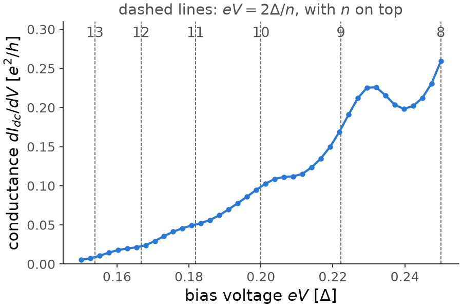
The figure is the snippet, with its 40 voltages, and it runs in about three minutes. The window from \(0.15\Delta\) to \(0.25\Delta\) is deep inside the gap, where the current is carried by Andreev processes of order \(n=8\) to \(13\). The conductance is small, from \(0.005\) to \(0.26\) in units of \(e^2/h\), and it is not smooth. It has a peak of \(0.23\) at \(0.23\Delta\), just above \(2\Delta/9\), then a minimum of \(0.20\) at \(0.24\Delta\), and it rises again towards \(2\Delta/8=0.25\Delta\). There is a shoulder at \(0.21\Delta\), just above \(2\Delta/10\), and weaker ones near \(2\Delta/11\) and \(2\Delta/12\). So each order \(n\) gives a feature close to \(2\Delta/n\), and the features are broad because the transparency, \(0.5\), is not small.

Code of this figure (documentation/figures/transport_finitev.py)

import style
from pyqula import geometry
from pyqula import heterostructures
import numpy as np
g = geometry.chain() # create the geometry
h = g.get_hamiltonian() # create the Hamiltonian
h1 = h.copy() ; h1.add_swave(0.1) # left superconducting lead
h2 = h.copy() ; h2.add_swave(0.1) # right superconducting lead
HT = heterostructures.build(h1,h2) # junction between the two superconductors
HT.set_coupling(0.5) # set the normal transparency of the weak link
es = np.linspace(0.15,0.25,40)*0.1 # bias energies
Gs = HT.didv(energies=es, nmax_max=40) # dI/dV curve
for (e,G) in zip(es,Gs): print(e,G)

def draw(ax, c):
    for n in range(8,14): # MAR features at eV = 2 Delta/n
        ax.axvline(2/n, color=c.ink2, lw=0.8, ls="--")
        ax.text(2/n, 0.29, f"{n}", color=c.ink2, ha="center")
    ax.set_title(r"dashed lines: $eV=2\Delta/n$, with $n$ on top", color=c.ink2)
    ax.plot(es/0.1, Gs, "o-", color=c.blue, ms=4)
    ax.set_ylim(0, 0.31)
    ax.set_xlabel(r"bias voltage $eV$ [$\Delta$]")
    ax.set_ylabel(r"conductance $dI_{dc}/dV$ [$e^2/h$]")

style.save(draw, "transport_finitev")

A superconducting STM tip

A LocalProbe is an STM tip, a semi-infinite chain coupled to one site of an infinite sample. The tip and the sample play the role of the two leads, and T is the hopping between them. The choice of method is the same as above: the scattering formula by default, and the Floquet-Keldysh current when both tip and sample are superconducting. For a normal tip the two methods agree, because the tip is grounded in both.

Besides the conductance, we compute the decay rate \(\kappa\). In STM, the conductance changes with the tip height through the transparency \(T\), and the exponent of this power law depends on how many electrons are transferred in each process. pyqula computes

\[\kappa = \frac{d\ln G_S/d\ln T}{d\ln G_N/d\ln T},\]

the ratio between the exponent with the superconductor and the exponent of the same junction with the pairing removed. In the tunnel limit \(G_N\propto T^2\). A single quasiparticle also gives \(G_S\propto T^2\), so \(\kappa=1\), while Andreev reflection transfers two electrons, \(G_S\propto T^4\), and \(\kappa=2\). So \(\kappa\) tells you which process carries the current at each energy, and it is measured by changing the tip height.

from pyqula import geometry
from pyqula.transporttk.localprobe import LocalProbe

g = geometry.chain()
h = g.get_hamiltonian() ; h.shift_fermi(1.) ; h.add_swave(0.1) # SC sample
lead = geometry.chain().get_hamiltonian() ; lead.shift_fermi(1.) ; lead.add_swave(0.1) # SC probe
lp = LocalProbe(h,lead=lead,delta=1e-3)
lp.T = 0.3 # reference transparency
G = lp.didv(energy=0.25,nmax=4,nmax_max=60,tol=5e-4) # routed through Keldysh automatically
k = lp.get_kappa(energy=0.25,nmax=4,nmax_max=60,tol=5e-4)

G is the conductance and k the decay rate at voltage \(0.25\), which is above the combined gap \(2\Delta=0.2\) of tip and sample. The snippet takes about a minute, much more than with a normal tip, because each didv or get_kappa call solves several Floquet-Keldysh problems, and it is slowest deep inside the gap at small transparency. See examples/transport/decay_constant_keldysh/main.py for a runnable script with a coarse energy grid and few sidebands, and the notebooks 08_tunneling_contact_probe.ipynb (normal tip) and 09_mar_ac_josephson_sc_probe.ipynb (superconducting tip) in jupyter-notebooks/functionalities/quantum_transport/.

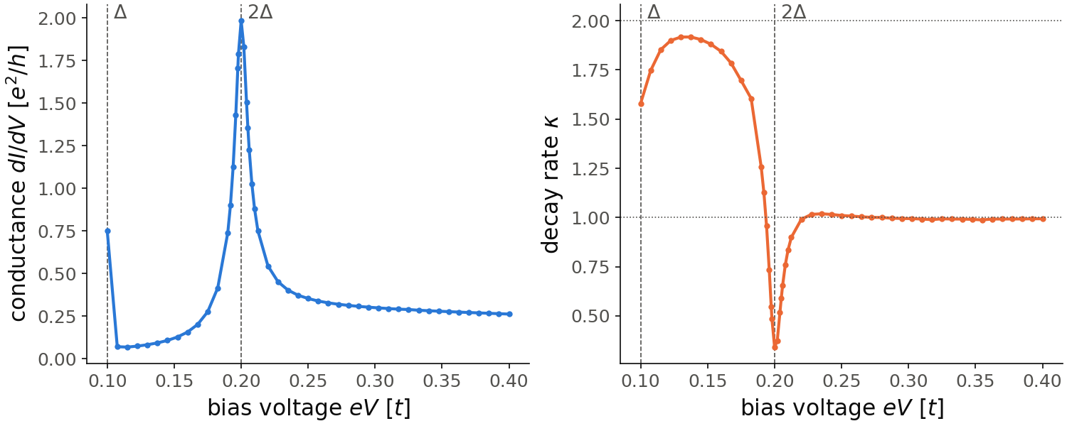
The figure repeats the snippet at 41 voltages from \(\Delta=0.1\) to \(0.4\), in steps of \(0.0075\), and at 11 more voltages between \(0.19\) and \(0.21\), around the peak at \(2\Delta\). It takes about 20 minutes. On the left, the conductance has its largest peak, \(1.98\,e^2/h\), at \(eV=0.2\), the sum of the gaps of tip and sample, where the coherence peaks of the two densities of states meet. The peak is narrow, its half width is about \(0.008\), so it needs the finer grid. A second peak, \(0.75\,e^2/h\), is at \(eV=\Delta\), the voltage \(2\Delta/2\) of the first Andreev reflection. Between the two the conductance is small, \(0.07\) to \(0.41\,e^2/h\). Above \(2\Delta\) it goes down to \(0.26\,e^2/h\) at \(eV=0.4\), the tunneling between the two continua.

On the right, \(\kappa\) is between \(0.99\) and \(1.02\) above \(eV=0.22\), so a single quasiparticle carries the current there. Between \(\Delta\) and \(2\Delta\), \(\kappa\) grows to \(1.92\) at \(eV\approx0.13\), close to 2: the current comes from Andreev reflection, which transfers two electrons. Near \(2\Delta\) it drops, and at \(2\Delta\) itself \(\kappa=0.34\), below one, because the peak of the conductance there grows more slowly with \(T\) than the normal conductance.

These values need converged sidebands. With tol=5e-4 and nmax_max=60, as in the snippet, the conductance and \(\kappa\) change by less than \(0.5\%\) with respect to tol=2e-3 and nmax_max=40. A looser tolerance is not enough: with tol=5e-2 and nmax_max=12 the conductance at \(eV=0.25\) is 7% too small, and inside the gap \(\kappa\) comes out as large as \(6\), while the converged value is below 2. With tol=2e-3 one point, \(eV=0.2725\), still came out at half its converged value. At a loose tolerance, get_kappa can also stop with an error, when the conductance changes sign between the two transparencies it needs, and the error asks for a tighter tol or a larger nmax_max. The figure starts at \(\Delta\): below it the higher orders of multiple Andreev reflection need more sidebands, and we did not converge those points.

Code of this figure (documentation/figures/transport_stmtip.py)

import numpy as np
import style
from pyqula import geometry
from pyqula.transporttk.localprobe import LocalProbe

g = geometry.chain()
h = g.get_hamiltonian() ; h.shift_fermi(1.) ; h.add_swave(0.1) # SC sample
lead = geometry.chain().get_hamiltonian() ; lead.shift_fermi(1.) ; lead.add_swave(0.1) # SC probe
lp = LocalProbe(h,lead=lead,delta=1e-3)
lp.T = 0.3 # reference transparency
es = np.linspace(0.1,0.4,41) # voltages from Delta up, in steps of 0.0075
es = np.unique(np.round(np.concatenate([es,np.linspace(0.19,0.21,11)]),6)) # and a finer grid around 2 Delta
G = lp.didv(energies=es,nmax=4,nmax_max=60,tol=5e-4) # routed through Keldysh automatically
k = lp.get_kappa(energies=es,nmax=4,nmax_max=60,tol=5e-4)
for (e,Ge,ke) in zip(es,G,k): print(e,Ge,ke)

def draw(ax, c):
    for a in ax:
        for (x,name) in [(0.1,r"$\Delta$"),(0.2,r"$2\Delta$")]:
            a.axvline(x, color=c.ink2, lw=0.8, ls="--")
            a.text(x, 1.0, " "+name, color=c.ink2, va="top",
                   transform=a.get_xaxis_transform())
        a.set_xlabel(r"bias voltage $eV$ [$t$]")
    ax[0].plot(es, G, "o-", color=c.blue, ms=3)
    ax[0].set_ylabel(r"conductance $dI/dV$ [$e^2/h$]")
    ax[1].plot(es, k, "o-", color=c.orange, ms=3)
    for kappa in [1,2]: # single quasiparticle, and Andreev reflection
        ax[1].axhline(kappa, color=c.ink2, lw=0.8, ls=":")
    ax[1].set_ylabel(r"decay rate $\kappa$")

style.save(draw, "transport_stmtip", npanels=2)

get_kappa also takes a temperature temp, and then every conductance is the thermal average at that temperature. Like didv, it takes a single energy or an array energies=[...]:

k = lp.get_kappa(energies=[0.1,0.25,0.4],temp=0.02,nmax=4,nmax_max=12,tol=5e-2)

HT.get_kappa() of a junction takes the same temp and energies.