Quasiparticle interference

In this page we compute what a single defect does to the local density of states of a two-dimensional system. A defect scatters an electron from a state with momentum \(\mathbf k\) to a state with momentum \(\mathbf k'\) on the same constant-energy contour. The incoming and the scattered waves interfere, so the local density of states around the defect oscillates with wavevector \(\mathbf q = \mathbf k' - \mathbf k\). The Fourier transform of these oscillations at each energy is called the quasiparticle interference (QPI) pattern. In an experiment, it is obtained by STM as the Fourier transform of a conductance map \(dI/dV(\mathbf r,V)\). It shows the constant-energy contours of the band structure, and which pairs of states the defect connects.

QPI from the spectral function

The simplest estimate of the QPI pattern is the autocorrelation of the momentum-resolved spectral function,

\[ P(\mathbf q,\omega) = \sum_{\mathbf k} A(\mathbf k,\omega)\,A(\mathbf k+\mathbf q,\omega) , \]

where \(A(\mathbf k,\omega)\) is the spectral weight at momentum \(\mathbf k\) and energy \(\omega\), broadened with a Lorentzian of width \(\delta\) (see Spectral functions). It counts all the pairs of states at energy \(\omega\) separated by \(\mathbf q\), so it is large for a \(\mathbf q\) that connects two flat, parallel parts of the contour. This is mode="pm" of h.get_qpi(), for 2D Hamiltonians:

import numpy as np
from pyqula import geometry
g = geometry.triangular_lattice()
h = g.get_hamiltonian(has_spin=False)
(qs,es,qpi) = h.get_qpi(mode="pm",nk=200,delta=1e-1,energies=np.linspace(-6.,6.,100)) # QPI at each energy

qs contains the wavevectors \(\mathbf q\), one per row, es the energies, and qpi the intensity, with one row per energy and one column per wavevector. So one row of qpi, plotted over qs, is the QPI map of an STM measurement at that energy. The band of the triangular lattice goes from \(-3t\) at K and K' to \(6t\) at \(\Gamma\). So near the top of the band the contour is a small circle of radius \(k_F\) around \(\Gamma\), and the QPI map is a disk of radius \(2k_F\), since \(2k_F\) is the largest momentum that connects two points of the circle. Near the bottom of the band the contour is two small pockets, around K and K'. The same maps are written to the folder MULTIQPI/, one file per energy, with the density of states in DOS.OUT, unless write=False is given.

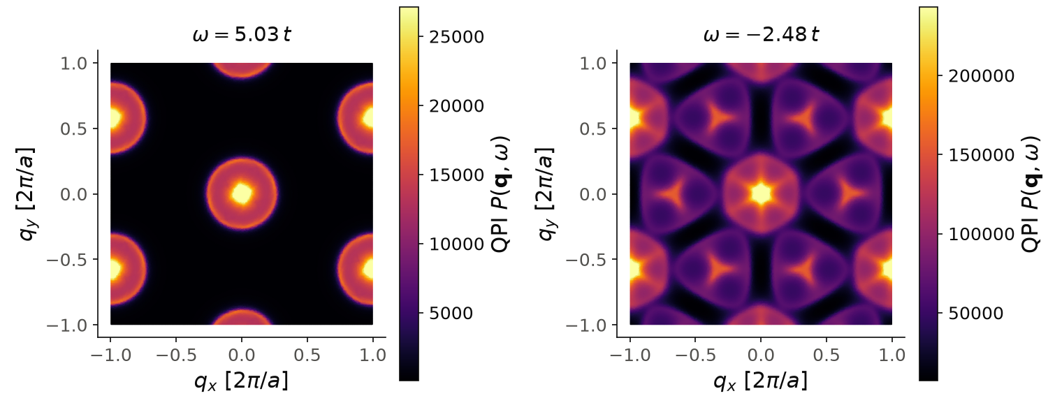
The wavevectors are Cartesian, in units of \(2\pi/a\), and the color scale stops at the 99th percentile, because the peak at \(\mathbf q=0\) is much larger than the rest. With this sign of the hopping, the band of the triangular lattice goes from \(-3t\) at K to \(6t\) at \(\Gamma\), so the small circle around \(\Gamma\) is at the top of the band. At \(\omega=5.03t\) (left) the contour is a circle of radius \(k_F\approx 0.13\) and the QPI map is a disk of radius \(0.26\), which is \(2k_F\), repeated at every reciprocal lattice vector. At \(\omega=-2.48t\) (right), near the bottom of the band, the contour is two small pockets around K and K'. The map has a disk at \(\mathbf q=0\), from the scattering inside one pocket, and bright features at the K points of \(\mathbf q\), from the scattering between the two pockets. The pockets are small, so they need a dense k-mesh: with nk=50 the right map is noisy, and the maps at nk=200 and nk=300 agree within one percent. With a smaller \(\delta\), increase nk again.

Code of this figure (documentation/figures/qpi_pm.py)

import numpy as np
import style
from pyqula import geometry

g = geometry.triangular_lattice()
h = g.get_hamiltonian(has_spin=False)
(qs,es,qpi) = h.get_qpi(mode="pm",nk=200,delta=1e-1,energies=np.linspace(-6.,6.,100)) # QPI at each energy

def draw(ax, c):
    for a, e0 in zip(ax, [5.0, -2.5]): # near the top and near the bottom of the band
        i = np.argmin(np.abs(es-e0)) # the energy closest to e0
        im = a.tripcolor(qs[:,0], qs[:,1], qpi[i], cmap=c.cmap, shading="gouraud",
                vmax=np.percentile(qpi[i],99)) # the q=0 peak saturates
        style.colorbar(im, a, r"QPI $P(\mathbf{q},\omega)$")
        a.set_title(r"$\omega=%.2f\,t$" % es[i])
        a.set_aspect("equal")
        a.set_xlabel(r"$q_x$ [$2\pi/a$]")
        a.set_ylabel(r"$q_y$ [$2\pi/a$]")

style.save(draw, "qpi_pm", npanels=2)

The keywords are

• energies: the energies \(\omega\).
• nk: number of k-points per direction.
• delta: the broadening \(\delta\).
• mode: "pm", the autocorrelation above, or "response" (default), a nesting function of the clean bands, defined below.
• operator: with "unfold", the spectral function of a supercell is unfolded to the primitive Brillouin zone (mode="pm" only).
• nunfold: the linear size of the supercell for the unfolding, as in g.get_supercell(): \(n\) for an \(n\times n\) supercell, np.sqrt(3) for a \(\sqrt3\times\sqrt3\) one.
• write: False to return the maps without writing files.

mode="response" uses only the energies of the bands, not the wavefunctions,

\[ R(\mathbf q,\omega) = \sum_{\mathbf k,\alpha,\beta} \Theta(\omega-\epsilon_{\mathbf k+\mathbf q,\alpha})\, \Theta(\epsilon_{\mathbf k,\beta}-\omega)\, \frac{\delta}{(\epsilon_{\mathbf k+\mathbf q,\alpha}-\epsilon_{\mathbf k,\beta})^2+\delta^2} , \]

which counts pairs of states, one below and one above \(\omega\), with almost the same energy. It is a measure of the nesting of the contour at energy \(\omega\). It is cheaper, but it ignores the form factors of the wavefunctions, and it does not accept an operator or unfolding. mode="pm" uses the real spectral weight of the system, defect included, and it is the one to use for a real scatterer.

The realistic case is a single point defect in a supercell, with the QPI unfolded back to the Brillouin zone of the primitive cell. The supercell must be built with store_primal=True, so that the primitive cell is known for the unfolding:

import numpy as np
from pyqula import geometry
g0 = geometry.honeycomb_lattice()
ns = 2
g = g0.get_supercell(ns,store_primal=True)
h = g.get_hamiltonian(has_spin=False)
h.add_onsite(lambda r: 100.0 if np.linalg.norm(r-g.r[0])<1e-1 else 0.0) # a strong point defect

h.get_qpi(mode="pm",delta=1e-2,operator="unfold",nsuper=2,nk=140,nunfold=ns)

This calculation is expensive. mode="pm" diagonalizes the Hamiltonian on an nk x nk mesh and then computes the autocorrelation, so nk=140 takes minutes. Use nk=60 (about 40 seconds) to prepare the calculation, and a large nk only for the final result, since nk sets the resolution in \(\mathbf q\).

See examples/2d/multiqpi/main.py (clean system, mode="pm") and examples/2d/multiqpi_unfold/main.py (defect in a supercell, unfolded) for runnable scripts.

QPI from a real-space impurity

h.get_qpi_impurity() does the calculation in the same way as the experiment. It builds a supercell of h, puts one or more impurities in it, computes the local density of states \(D(\mathbf r,\omega)\) around them (see Local density of states), and takes its Fourier transform,

\[ \textrm{QPI}(\mathbf q,\omega) = \left| \sum_{\mathbf r} e^{-i\mathbf q\cdot\mathbf r}\, D(\mathbf r,\omega) \right| . \]

So here the interference of the scattered waves is included exactly, for the impurity potential you choose:

from pyqula import geometry
g = geometry.honeycomb_lattice()
h = g.get_hamiltonian(has_spin=False)
r,ldos_r,q,qpi_q = h.get_qpi_impurity(nsuper=10,
        impurities=[{"position": [0.,0.,0.], "onsite": 3.0}],
        energies=0.3,num_waves=60,nk=2,delta=0.2)

r and ldos_r are the positions of the sites and the local density of states on them, the real-space map. q and qpi_q are the wavevectors and the QPI intensity, its Fourier transform.

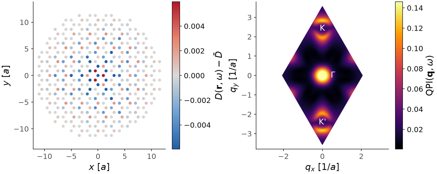
For the figure we take a much larger supercell, nsuper=69, so that the \(\mathbf q\) mesh is fine and the oscillations decay well inside the supercell. The size is a multiple of three, because only then the K points are on the \(\mathbf q\) mesh. With such a large supercell one k-point is enough (nk=1), and we can take a smaller broadening, \(\delta=0.1t\). We ask for all the states with num_waves, which is a full diagonalization of 9522 sites, and it takes about 3 minutes. With nsuper=48 the maps are the same within a few percent. Lengths are in units of the first-neighbor distance \(a\). On the left, the change of the local density of states at \(\omega=0.3t\) with respect to its mean, within \(12a\) of the impurity. The color scale stops at the 95th percentile, so that the impurity site, where the density drops, does not hide the rest. You see the Friedel oscillations around the impurity, with a period of \(3a\) along \(x\), and they decay with the distance. On the right, the QPI intensity over the \(69\times 69\) points of the mesh, which cover one Brillouin zone. The point \(\mathbf q=0\) is left out, since it is the mean density and it is about 4200 times larger than the rest. The brightest feature is then the disk around \(\Gamma\), from the scattering inside one valley. Around K and K', at \(|\mathbf q|\approx 2.4/a\), there is a ring of radius about \(0.4/a\), which is \(2k_F\) of the Dirac cone at this energy, brightest along the line to \(\Gamma\). This is the scattering between the two valleys, and it gives the period of \(3a\) in real space. For larger maps, or for a single impurity in an infinite system, use the T-matrix, described in QPI from the T-matrix: it gives the same result as this calculation with nk=1 and nsuper equal to the nk of the T-matrix, at a much lower cost.

Code of this figure (documentation/figures/qpi_impurity.py)

import numpy as np
import style
from pyqula import geometry

g = geometry.honeycomb_lattice()
h = g.get_hamiltonian(has_spin=False)
ns = 69 # a multiple of three, so the K points are on the q mesh
r,ldos_r,q,qpi_q = h.get_qpi_impurity(nsuper=ns,
        impurities=[{"position": [0.,0.,0.], "onsite": 3.0}],
        energies=0.3,num_waves=2*ns**2, # all the states, a full diagonalization
        nk=1,delta=0.1)

ldos_r, qpi_q = np.ravel(ldos_r), np.ravel(qpi_q) # one energy
r0 = r[np.argmin(ldos_r)] # the impurity site, where the density drops
q0 = np.argmin(np.linalg.norm(q,axis=1)) # q=0 holds the mean LDOS
qpi_q[q0] = np.nan # leave it out of the color scale
ok = ~np.isnan(qpi_q)
K = 4*np.pi/(3*np.sqrt(3)) # |K| for a first-neighbor distance a=1

def draw(ax, c):
    dl = ldos_r - ldos_r.mean() # the change around the mean
    w = np.linalg.norm(r-r0,axis=1) < 12 # a window around the impurity
    m = np.percentile(np.abs(dl[w]),95) # the impurity site itself saturates
    sc = ax[0].scatter(r[w,0]-r0[0], r[w,1]-r0[1], c=dl[w], s=16,
            cmap=c.diverging, vmin=-m, vmax=m)
    style.colorbar(sc, ax[0], r"$D(\mathbf{r},\omega)-\bar D$")
    ax[0].set_xlabel("$x$ [$a$]")
    ax[0].set_ylabel("$y$ [$a$]")
    im = ax[1].tripcolor(q[ok,0], q[ok,1], qpi_q[ok], cmap=c.cmap,
            shading="gouraud", vmax=np.percentile(qpi_q[ok],99))
    style.colorbar(im, ax[1], r"QPI$(\mathbf{q},\omega)$")
    for (x,y,s) in [(0.55,0,r"$\Gamma$"),(0,K,"K"),(0,-K,"K'")]: # K and K'
        ax[1].text(x, y, s, color="w", ha="center", va="center") # in the dark center of their ring
    ax[1].set_xlabel("$q_x$ [$1/a$]")
    ax[1].set_ylabel("$q_y$ [$1/a$]")
    for a in ax: a.set_aspect("equal", adjustable="datalim")

style.save(draw, "qpi_impurity", npanels=2)

The keywords are

• nsuper: size of the supercell, a number or (n1,n2).
• impurities: a list of impurities. Each one is an onsite potential, {"position": [x,y,z], "onsite": v} (or {"index": i, "onsite": v} for a site of the supercell), or a vacancy, {"position": [x,y,z], "vacancy": True}.
• energies: one energy or an array of energies.
• num_waves: a first guess for the number of eigenstates computed near each energy. It is increased automatically when needed.
• nk, delta: as in h.get_ldos().

A vacancy is modeled as a very large onsite potential on the site, which in practice removes the site from the low-energy states.

The wavevectors q are the \(n_1\times n_2\) points that are commensurate with the supercell, and they cover the whole Brillouin zone of the primitive cell. So nsuper sets the resolution in \(\mathbf q\), not the range. Only these points are free of finite-size artifacts: at any other \(\mathbf q\), even a clean supercell would give a signal. No unfolding is needed here, because the Fourier transform is done directly on the real-space density.

See examples/2d/qpi_realspace_impurity/main.py for a runnable script that plots the real-space map and the QPI, and jupyter-notebooks/functionalities/spectral_functions/07_qpi_maps.ipynb for an executed notebook.

QPI from the T-matrix

We will now see how to compute the QPI of a single impurity in an infinite system, without a supercell. The way we do this is with the T-matrix. We take the clean Hamiltonian \(H_0\) and one impurity \(V\), which acts only inside the unit cell at the origin. The Green's function of the clean system is

\[ G_0(\mathbf k,\omega) = \left[\omega + i\delta - H_0(\mathbf k)\right]^{-1} , \]

where \(H_0(\mathbf k)\) is the Bloch Hamiltonian and \(\delta\) the broadening. The impurity scatters the electrons many times. The sum of all these scattering events is the T-matrix,

\[ T(\omega) = V\left[1 - G_0(\omega)\,V\right]^{-1}, \qquad G_0(\omega) = \frac{1}{N}\sum_{\mathbf k} G_0(\mathbf k,\omega) , \]

where \(G_0(\omega)\) is the local Green's function of the unit cell and \(N\) the number of k-points. Because the impurity is local, \(T\) does not depend on momentum. The Green's function with the impurity is \(G = G_0 + G_0 T G_0\), so the change of the local density of states has the Fourier transform

\[ \delta\rho(\mathbf q,\omega) = -\frac{1}{2\pi i}\sum_a e^{-i\mathbf q\cdot\boldsymbol\tau_a} \left[\Lambda_{aa}(\mathbf q,\omega) - \Lambda_{aa}^*(-\mathbf q,\omega)\right], \qquad \Lambda(\mathbf q,\omega) = \frac{1}{N}\sum_{\mathbf k} G_0(\mathbf k,\omega)\,T(\omega)\,G_0(\mathbf k-\mathbf q,\omega) , \]

where \(a\) runs over the orbitals of the unit cell and \(\boldsymbol\tau_a\) is the position of the site of orbital \(a\), so the result is the Fourier transform of a real-space map, as in STM. This is the formalism of the review by Rhodes, Kohsaka, Hanaguri, Marques and Wahl (arXiv:2607.22487). For a superconductor, only the electron part of the Nambu Green's function enters the trace. The QPI intensity is \(|\delta\rho(\mathbf q,\omega)|\).

When the impurity is weak, \(T\approx V\). This is called the Born approximation, and it is the first order in \(V\). For a point impurity in a single-band model with inversion symmetry, the expression above becomes \(\delta\rho = -\frac{1}{\pi}\textrm{Im}[T\,\Lambda_0(\mathbf q)]\), where \(\Lambda_0\) is the sum of \(G_0(\mathbf k)G_0(\mathbf k-\mathbf q)\). In the Born approximation \(T=V\) is real, so only \(\textrm{Im}\,\Lambda_0\) enters. A strong impurity has a complex \(T\), so \(\textrm{Re}\,\Lambda_0\) enters too, and the shape of the pattern changes, not only its size.

This is mode="tmatrix" of h.get_qpi(), and mode="born" for the Born approximation. The impurity is given with impurity:

from pyqula import geometry
g = geometry.square_lattice()
h = g.get_hamiltonian(has_spin=False)
(qs,es,qpi) = h.get_qpi(mode="tmatrix",impurity=5.0,nk=120,nsuper=2,
        delta=1e-1,energies=[-1.0]) # a strong point impurity

As for the other modes, qs contains the wavevectors, one per row, in units of the reciprocal lattice vectors, es the energies, and qpi the intensity, with one row per energy and one column per wavevector. Here \(\delta\rho\) contains only the change due to the impurity, so the point \(\mathbf q=0\) is the change of the total density of states, and it is not much larger than the rest.

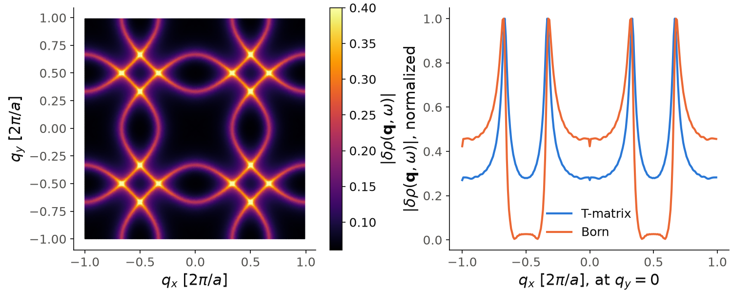
The band of the square lattice goes from \(-4t\) at M to \(4t\) at \(\Gamma\). At \(\omega=-t\) the contour is a rounded square around M, with a radius \(k_F=1/3\) along the axes, in units of \(2\pi/a\). On the left, the QPI map of an impurity with \(V=5t\). You see a rounded square of radius \(2k_F=2/3\) around every reciprocal lattice vector, so the lines cross the \(q_x\) axis at \(q_x=\pm 1/3\) and \(\pm 2/3\). These are the vectors that connect the parallel sides of the contour, which give the strongest interference. On the right, the cut at \(q_y=0\), each curve divided by its maximum. The peaks are at the same \(\mathbf q\) for the T-matrix and for the Born approximation, since they come from the contour. The background is different: between \(q_x=1/3\) and \(2/3\) the Born result drops almost to zero, while the T-matrix stays at about \(0.3\) of the peak. For this impurity \(T\approx(1.1-1.1i)\,t\), so the real part of \(\Lambda_0\) enters with the same weight as the imaginary part.

Code of this figure (documentation/figures/qpi_tmatrix.py)

import numpy as np
import style
from pyqula import geometry

g = geometry.square_lattice()
h = g.get_hamiltonian(has_spin=False)
(qs,es,qpi) = h.get_qpi(mode="tmatrix",impurity=5.0,nk=120,nsuper=2,
        delta=1e-1,energies=[-1.0]) # a strong point impurity
(qs,es,qpib) = h.get_qpi(mode="born",impurity=5.0,nk=120,nsuper=2,
        delta=1e-1,energies=[-1.0]) # its Born approximation

cut = np.abs(qs[:,1])<1e-9 # the line q=(q_x,0)
order = np.argsort(qs[cut,0])

def draw(ax, c):
    im = ax[0].tripcolor(qs[:,0], qs[:,1], qpi[0], cmap=c.cmap, shading="gouraud",
            vmax=np.percentile(qpi[0],99.5))
    style.colorbar(im, ax[0], r"$|\delta\rho(\mathbf{q},\omega)|$")
    ax[0].set_aspect("equal")
    ax[0].set_xlabel(r"$q_x$ [$2\pi/a$]")
    ax[0].set_ylabel(r"$q_y$ [$2\pi/a$]")
    for (y,col,lab) in [(qpi[0],c.blue,"T-matrix"),(qpib[0],c.orange,"Born")]:
        y = y[cut][order]
        ax[1].plot(qs[cut,0][order], y/np.max(y), color=col, label=lab)
    ax[1].set_xlabel(r"$q_x$ [$2\pi/a$], at $q_y=0$")
    ax[1].set_ylabel(r"$|\delta\rho(\mathbf{q},\omega)|$, normalized")
    ax[1].legend()

style.save(draw, "qpi_tmatrix", npanels=2)

The keywords are

• impurity: a number, an onsite potential on the first site of the unit cell; a list with one onsite potential per site of the cell; or a matrix with the dimension of the Hamiltonian of the cell, for example a magnetic impurity \(V\,\mathbf m\cdot\boldsymbol\sigma\) in a spinful system.
• nk: number of k-points per direction. The wavevectors are on the same mesh, so nk also sets the resolution in \(\mathbf q\).
• nsuper: number of Brillouin zones per direction covered by qs.
• energies, delta, write: as in mode="pm".

The sum over k-points on an nk x nk mesh is the same as one impurity in a periodic system of nk x nk unit cells. So the result is exact for that system, and it is the same as h.get_qpi_impurity() with nsuper=nk and nk=1, at every \(\mathbf q\) except \(\mathbf q=0\), where the real-space map also contains the density of states of the clean system. For a single impurity in an infinite system, nk must be larger than the length over which the Friedel oscillations decay, which is about \(v_F/\delta\) in units of the lattice constant, where \(v_F\) is the Fermi velocity. In the figure \(v_F\approx 1.7\,ta\) and \(\delta=0.1t\), so this is about 20 unit cells, and nk=120 is enough. With a smaller \(\delta\), increase nk.

The impurity matrix also lets you check a selection rule. With time-reversal symmetry, the two states of a Kramers pair give opposite contributions for a magnetic impurity. So in the Born approximation a magnetic impurity gives no QPI at all, even with a Rashba spin-orbit coupling. The T-matrix gives a signal at second order in \(V\). In the square lattice with a Rashba coupling of \(0.4t\), at \(\omega=-t\), the largest QPI intensity of a magnetic impurity with \(V=0.3t\) is about 14 times weaker than the one of a potential impurity of the same strength, and about 3 times weaker for \(V=t\).

See examples/2d/qpi_tmatrix/main.py for a runnable script.