Kernel polynomial method

Exact diagonalization gives all the eigenstates, and its cost grows as the cube of the number of sites. For a system with \(10^5\) or \(10^6\) sites this is not possible, and also not needed: the density of states is a trace, and a trace can be computed without the eigenstates. The kernel polynomial method (KPM) does this. It expands the density of states in Chebyshev polynomials of the Hamiltonian, and only needs products of a vector with the sparse Hamiltonian, so its cost is linear in the number of sites.

The density of states of a large system

The Chebyshev polynomials \(T_m(x)\) are defined on \([-1,1]\), so we first rescale the Hamiltonian, \(\tilde H = H/s\), with a scale \(s\) larger than the largest energy. They obey the recursion

\[T_0(x)=1,\qquad T_1(x)=x,\qquad T_{m+1}(x)=2xT_m(x)-T_{m-1}(x).\]

The density of states at energy \(E\), with \(x=E/s\), is

\[ \rho(E) = \frac{1}{\pi s\sqrt{1-x^2}} \left[ g_0\mu_0 + 2\sum_{m\geq 1} g_m\,\mu_m\,T_m(x) \right], \qquad \mu_m = {\rm Tr}\, T_m(\tilde H) . \]

The \(\mu_m\) are the moments. They are computed with the recursion above, applied to a vector: \(|v_{m+1}\rangle = 2\tilde H|v_m\rangle - |v_{m-1}\rangle\), so each moment costs one sparse matrix-vector product. The trace is estimated with random vectors \(|r\rangle\), as \({\rm Tr}\,A \approx \frac{1}{R}\sum_{r=1}^{R}\langle r|A|r\rangle\), and the error goes down as \(1/\sqrt R\). The series is cut after \(N\) moments, and this creates oscillations (Gibbs oscillations). The factors \(g_m\) of the Jackson kernel remove them,

\[ g_m = \frac{(N-m+1)\cos\frac{\pi m}{N+1} + \sin\frac{\pi m}{N+1}\cot\frac{\pi}{N+1}}{N+1}, \]

and the price is that every eigenvalue becomes a peak of finite width, nearly a Gaussian. In pyqula \(N=2n_{\rm pol}\), with \(n_{\rm pol}\) the number of polynomials, because each step of the recursion gives two moments.

The KPM density of states is h.get_dos() with mode="KPM":

from pyqula import geometry
import numpy as np
g = geometry.chain()
g = g.get_supercell(100000) # a big supercell
g.dimensionality = 0
h = g.get_hamiltonian(is_sparse=True,has_spin=False)
(x,y) = h.get_dos(mode="KPM",
            energies=np.linspace(-3.0,3.0,601), # energies
            delta=1e-2, # energy resolution, half width of the peak of a level
            ntries=40 # number of random vectors for the stochastic trace
            )

x is the energy grid and y the density of states, the same quantity that exact diagonalization would give for this chain of \(10^5\) sites. For a chain you see the one-dimensional van Hove singularities at \(E=\pm2\). A sparse Hamiltonian (is_sparse=True) is the natural choice, since the method never needs the dense matrix. This snippet takes about one minute.

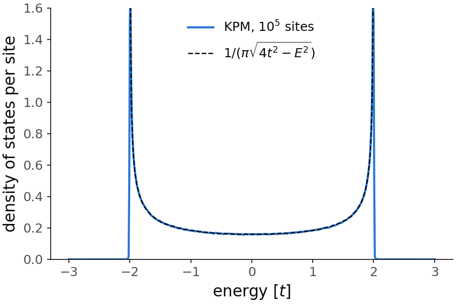
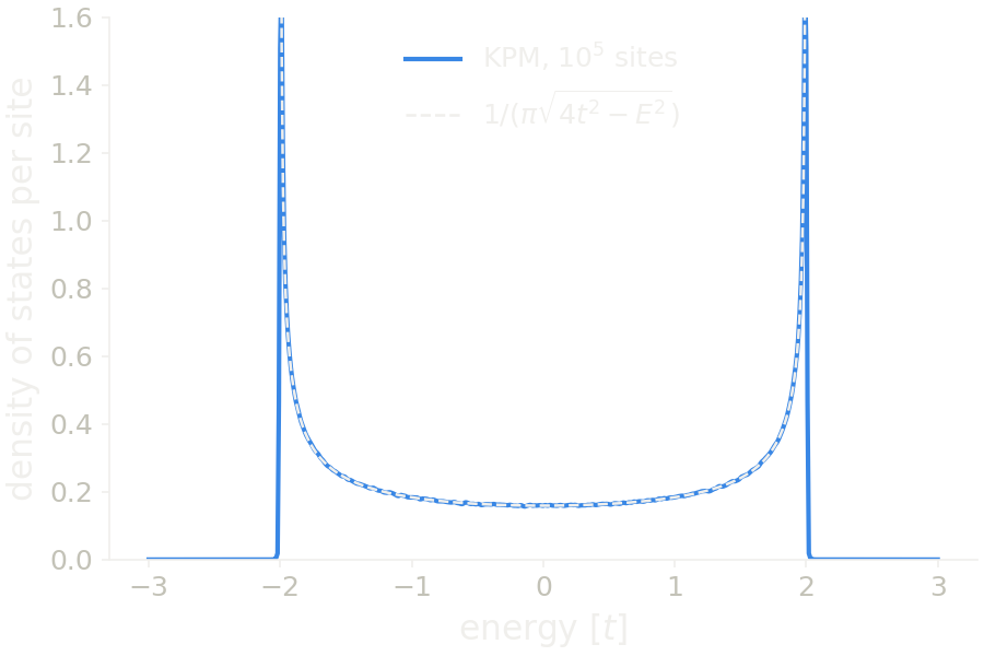
The KPM density of states, divided by the number of sites (blue), follows the one of the infinite chain, \(1/(\pi\sqrt{4t^2-E^2})\) (dashed), and the two curves lie on top of each other. You see the two van Hove peaks at \(E=\pm2\), and the minimum \(1/(2\pi)=0.16\) at zero energy. Outside the band it is zero. Inside the band, the only error is the noise of the stochastic trace. Each random vector already averages over the \(N\) sites, so the noise goes down as \(1/\sqrt{NR}\). For \(|E|<1.5\) it is \(0.5\%\) on average and at most \(2\%\) at a single energy. With 3000 sites and 10 random vectors it was \(5\%\) on average and up to \(18\%\), and with \(3\times10^5\) sites and 80 vectors it is \(0.2\%\), so the curve does not change any more at the scale of the figure.

At the band edges the error is of another kind. The exact density of states diverges as \(1/\sqrt{2-|E|}\), and the KPM curve cannot follow it, because every level is a peak of half width delta. So the divergence becomes a finite peak, \(1.73\) per site at \(E=\pm1.99\), and just inside the edge the curve is a little above the exact one. This does not improve with more sites or more random vectors. Only a smaller delta helps: with delta=5e-3 the peak is \(2.15\), and it keeps growing as delta goes down.

Code of this figure (documentation/figures/kpm_dos.py)

import style
from pyqula import geometry
import numpy as np
np.random.seed(1) # the same random vectors in every run
g = geometry.chain()
g = g.get_supercell(100000) # a big supercell
g.dimensionality = 0
h = g.get_hamiltonian(is_sparse=True,has_spin=False)
(x,y) = h.get_dos(mode="KPM",
            energies=np.linspace(-3.0,3.0,601), # energies
            delta=1e-2, # energy resolution, half width of the peak of a level
            ntries=40 # number of random vectors for the stochastic trace
            )
N = len(g.r) # number of sites
x0 = np.linspace(-1.999,1.999,400)
y0 = N/(np.pi*np.sqrt(4-x0**2)) # density of states of the infinite chain

x = np.array(x) ; inside = np.abs(x)<1.5 # far from the band edges
exact = 1/(np.pi*np.sqrt(4-x[inside]**2))
dev = np.abs(y[inside]/N/exact-1) # relative deviation from the infinite chain
print("deviation for |E|<1.5: mean",dev.mean(),"max",dev.max())
print("peak at the band edge:",y.max()/N,"at E =",x[np.argmax(y)])

def draw(ax, c):
    ax.plot(x, y/N, color=c.blue, label="KPM, $10^5$ sites")
    ax.plot(x0, y0/N, "--", color=c.ink, lw=1.2, label=r"$1/(\pi\sqrt{4t^2-E^2})$")
    ax.set_xlabel("energy [$t$]")
    ax.set_ylabel("density of states per site")
    ax.set_ylim(0, 1.6)
    ax.legend(loc="upper center")

style.save(draw, "kpm_dos")

Two numbers control the result:

• delta: the energy resolution, the half width at half maximum of the peak of a single level. It is the same width that delta gives as a Lorentzian in mode="ED", so the two curves can be compared. The method uses \(n_{\rm pol}\approx 1.85\,s/\delta\) polynomials, so a sharper density of states costs more. The KPM peak is nearly a Gaussian, about 1.5 times taller than the Lorentzian and without its long tails.
• ntries: the number of random vectors \(R\). The noise in y goes as \(1/\sqrt R\).

delta must be larger than the distance between levels, here \(2\pi t/N\approx 6\times10^{-5}\) in the middle of the band, otherwise y shows the single levels of the finite chain. The spectrum must be inside \([-s,s]\), since \(T_m(x)\) grows exponentially outside \([-1,1]\). The default is scale=10 in units of the hopping. A Hamiltonian with a larger spectrum, for example with a large onsite energy or exchange field, needs a larger scale. If scale is too small, the code raises a ValueError.

Green's functions between two sites

The same expansion also gives the Green's function between two sites \(i\) and \(j\) of this chain, without inverting a matrix. The function kpm.dm_ij_energy() gives

\[ \pi\,\langle i|\delta(E-H)|j\rangle = \pi\sum_n \psi_n(i)\psi_n^*(j)\,\delta(E-E_n) = \frac{i}{2}\left[G^R_{ij}(E)-G^A_{ij}(E)\right], \]

the spectral part of the Green's function:

from pyqula import kpm
(x,y) = kpm.dm_ij_energy(h.intra,npol=200,i=0,j=9,ne=1000)

For \(i=j\) it is \(\pi\) times the local density of states of site \(i\). For \(i\neq j\) it integrates to zero over all energies, because the eigenstates form a complete basis. Its integral up to the Fermi energy is \(\pi\) times the density matrix element \(\langle c^\dagger_j c_i\rangle\), so its sign along the energy axis tells which part of the spectrum correlates the two sites. Here npol is the number of polynomials \(n_{\rm pol}\), and each level becomes a peak of half width \(1.85\,s/n_{\rm pol}\), the inverse of the relation for delta above.

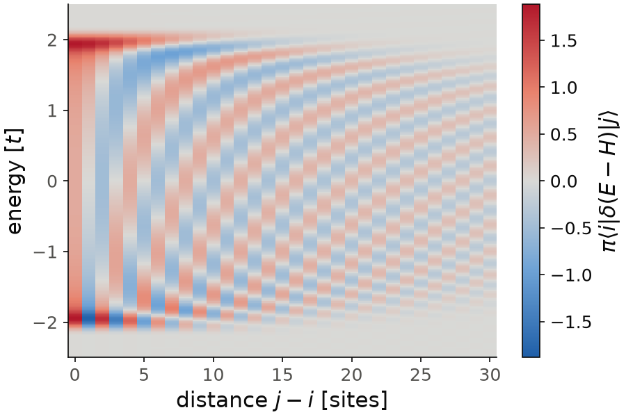
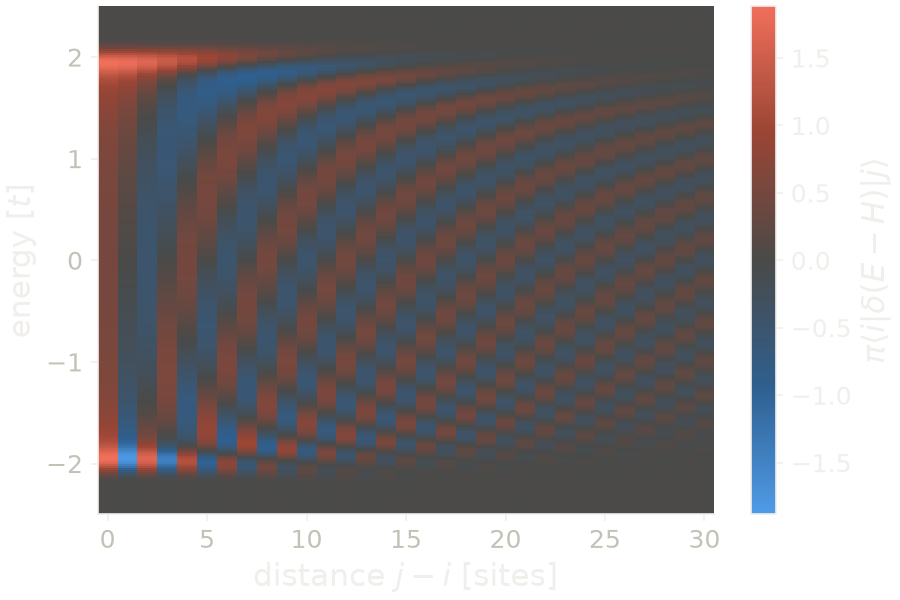
For the figure we take the site \(i=1500\), in the middle of the chain and far from its ends, and compute the same quantity for \(j=i\) to \(i+30\). The first column, \(j=i\), is \(\pi\) times the LDOS: \(0.50=\pi/(2\pi)\) at zero energy, with peaks at the band edges. At zero energy the value along the chain is \(0.5, 0, -0.5, 0, 0.5, \dots\), the oscillation \(\cos(k_F d)\) with \(k_F=\pi/2\). Further away the sign changes faster along the energy axis, and the finite resolution of 200 polynomials washes it out. The integral over all energies is \(\pi\) for \(j=i\) and zero for the other sites. The integral up to zero energy, divided by \(\pi\), is \(0.5\) for \(j=i\), the occupation of a site at half filling, and \(-0.318=-1/\pi\) for the first neighbor.

Code of this figure (documentation/figures/kpm_green.py)

import numpy as np
import style
from pyqula import geometry
g = geometry.chain()
g = g.get_supercell(3000) # a big supercell
g.dimensionality = 0
h = g.get_hamiltonian(is_sparse=True,has_spin=False)

from pyqula import kpm
(x,y) = kpm.dm_ij_energy(h.intra,npol=200,i=0,j=9,ne=1000)

js = range(1500,1531) # sites j, from the middle of the chain
gij = np.array([kpm.dm_ij_energy(h.intra,npol=200,i=1500,j=j,ne=1000)[1].real for j in js])

def draw(ax, c):
    vm = np.abs(gij).max()
    m = ax.pcolormesh(np.array(js)-1500, x, gij.T, cmap=c.diverging, vmin=-vm, vmax=vm,
                      shading="nearest")
    style.colorbar(m, ax, r"$\pi\langle i|\delta(E-H)|j\rangle$")
    ax.set_xlabel("distance $j-i$ [sites]")
    ax.set_ylabel("energy [$t$]")
    ax.set_ylim(-2.5, 2.5)

style.save(draw, "kpm_green")

The full Green's function, with its real part, comes from kpm.correlator0d(). It returns the energies, \({\rm Re}\,G^R_{ij}\) and \(-{\rm Im}\,G^R_{ij}\). With kernel="lorentz" each pole becomes a Lorentzian of half width \(1.5\,s/n_{\rm pol}\), which is the \(G^R_{ij}(E+i\delta)\) that a matrix inversion gives. The cutoff of the expansion leaves an error of about 10% on a sharp pole. The keyword lorentz_lambda, called \(\lambda\) here, reduces it. The half width is then \(\lambda s/(2n_{\rm pol})\), so for the same \(\delta\) you need \(n_{\rm pol}=\lambda s/(2\delta)\). The error falls roughly as \(e^{-\lambda}\). On a small chain it is 9% at the default \(\lambda=3\) and 0.3% at \(\lambda=8\).

See examples/0d/kpm_dos/main.py and examples/0d/kpm_correlator/main.py for runnable scripts, the second one with a comparison against the exact Green's function, and jupyter-notebooks/functionalities/chebyshev_kpm_algorithms/ for the local and non-local spectral functions of a system too large to diagonalize.

On a GPU

The Chebyshev moments of the same density of states can also be computed on a GPU, with the switch described in GPU. The keyword kpm_prec chooses single or double precision for the moments:

from pyqula import gpu
gpu.set_gpu(True) # Chebyshev moments on the GPU from now on
(x,y) = h.get_dos(mode="KPM",
            energies=np.linspace(-3.0,3.0,200),
            delta=1e-4,ntries=10,
            kpm_prec="single") # single precision moments

If there is no GPU, the same code runs on the CPU with a warning.

The local density of states of a large system

We now compute the local density of states of every site of a large system, which is the map that STM measures, with h.get_multildos() and h.get_ldos() in mode="KPM". The local density of states of orbital \(i\) is \(D(\omega,i)=\langle i|\delta(\omega-H)|i\rangle\). It has the same expansion as the total density of states, but with the moments of one orbital,

\[ D(\omega,i) = \frac{g_0\mu_0(i) + 2\sum_{m\geq 1} g_m\mu_m(i)\,T_m(\omega/s)}{\pi s\sqrt{1-(\omega/s)^2}}, \qquad \mu_m(i)=\langle i|T_m(H/s)|i\rangle , \]

so no random vectors are needed: the recursion starts from orbital \(i\).

Doing this recursion over the whole system for every orbital costs the square of the number of sites. pyqula avoids this. After \(m\) steps, the vector that started on orbital \(i\) has only reached the sites within \(m\) hops of \(i\). The \(2n_{\rm pol}\) moments only need \(n_{\rm pol}-1\) steps, because \(T_{2m}=2T_mT_m-T_0\) and \(T_{2m+1}=2T_{m+1}T_m-T_1\) give two moments per step. So the moments computed on the sites within \(n_{\rm pol}-1\) hops of \(i\) are exactly those of the whole system, and the full map costs a time linear in the number of sites.

from pyqula import geometry
import numpy as np
g = geometry.honeycomb_lattice().get_supercell(80) # 12800 sites
g.dimensionality = 0 # a finite island with zigzag edges
h = g.get_hamiltonian(is_sparse=True,has_spin=False) # keep it sparse
(x,y,es,ldos) = h.get_multildos(energies=np.linspace(-1.,1.,41), # energies
                    mode="KPM", # Chebyshev expansion of every site
                    delta=0.1, # energy resolution, half width of the peak of a level
                    write=False) # return the maps without writing them

ldos contains one map per energy, one row for each energy of es. All the rows come from the same moments, so 41 energies cost about the same as one. h.get_ldos(e=0.,mode="KPM",delta=0.1) gives only the map at zero energy. In this island the 318 sites at the zigzag edges, about 2.5% of all the sites, carry 56% of the weight at zero energy: these are the zigzag edge states. At \(E=\pm1\) the same sites carry only 1.4%. The sum of a map over the sites is the density of states at that energy, with the normalization of h.get_dos(mode="KPM"). The result is the same as the expansion over the whole island, up to roundoff.

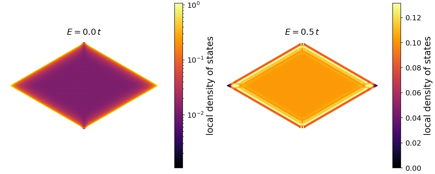
Both maps show the whole island, a rhombus with four zigzag edges. At zero energy (left) the color scale is logarithmic, because the map covers three decades. The outer sites of the edges are bright: these are the zigzag edge states. Their typical LDOS is \(1.1\), and \(2.8\) at the sharp corners, so they are saturated, since the color scale is cut at \(1.07\). Their weight decays into the island over a few rows, and the bulk is dark, with a typical LDOS of \(0.012\). At the two blunt corners the edge states are suppressed. At \(E=0.5\) (right, linear scale) the map is the opposite. The bulk is almost uniform, about \(0.10\), and the edge sites are no longer special: they carry \(2.4\%\) of the weight, about the same as their share of the sites. The brighter lines parallel to the edges are standing waves of the bulk states, reflected at the edge. The color scale is cut at \(0.13\), and the brightest sites of the map reach \(0.22\).

Code of this figure (documentation/figures/kpm_ldos.py)

import style
from pyqula import geometry
import numpy as np
g = geometry.honeycomb_lattice().get_supercell(80) # 12800 sites
g.dimensionality = 0 # a finite island with zigzag edges
h = g.get_hamiltonian(is_sparse=True,has_spin=False) # keep it sparse
(x,y,es,ldos) = h.get_multildos(energies=np.linspace(-1.,1.,41), # energies
                    mode="KPM", # Chebyshev expansion of every site
                    delta=0.1, # energy resolution, half width of the peak of a level
                    write=False) # return the maps without writing them

# the sites at the edge have two neighbors instead of three
edge = h.intra.getnnz(axis=1) < 3 # number of hoppings from each site
print("edge sites:",edge.sum(),"of",len(x))
for i in [20,30]: # E = 0 and E = 0.5
    m = ldos[i]
    print("E =",es[i],"edge weight:",m[edge].sum()/m.sum(),
          "bulk median:",np.median(m[~edge]),"edge median:",np.median(m[edge]),
          "max:",m.max())

from matplotlib.colors import LogNorm, Normalize
def draw(axs, c):
    for (ax,i) in zip(axs, [20, 30]): # E = 0 and E = 0.5
        m = ldos[i]
        o = np.argsort(m) # the brightest sites are drawn last, on top
        vmax = np.percentile(m, 99.5) # the brightest edge sites saturate
        if i==20: norm = LogNorm(vmin=vmax/1000, vmax=vmax) # three decades at E=0
        else: norm = Normalize(vmin=0, vmax=vmax)
        s = ax.scatter(x[o], y[o], c=m[o], s=4, lw=0, cmap=c.cmap, norm=norm)
        style.colorbar(s, ax, "local density of states")
        ax.set_title("$E=%.1f\\,t$" % es[i])
        ax.set_aspect("equal")
        ax.set_axis_off()

style.save(draw, "kpm_ldos", npanels=2)

The cost of one site is set by the resolution. A peak of half width \(\delta\) needs about \(1.85\,s/\delta\) polynomials, here 62, and the region of 61 hops around a site contains about 5700 sites of the honeycomb lattice. In two dimensions this region grows as \(n_{\rm pol}^2\), so halving \(\delta\) makes each site eight times more expensive. You can think of it in this way: with a resolution \(\delta\), a site only sees its environment up to a distance of about \(v/\delta\), where \(v\) is the velocity of the electrons, whatever the size of the sample.

The vector has almost no weight near the border of this region, so kpm_radius smaller than \(n_{\rm pol}\) gives a cheaper map that is still converged in practice. On a disordered honeycomb island of 20000 sites with npol=100, the map with kpm_radius=80, 70, 60 and 50 differs from the exact one by \(10^{-11}\), \(2\times10^{-7}\), \(5\times10^{-5}\) and \(10^{-3}\) of its largest value, and with 60 it takes about one third of the time. How small the radius can be depends on the velocity of the states, so you should converge it as you converge a k-mesh, by comparing two values.

The keywords are:

• delta: energy resolution, the half width at half maximum of the peak of a level, as in h.get_dos(mode="KPM").
• npol: number of polynomials, instead of delta; 200 if neither is given.
• kpm_radius: radius in hops of the region around each site; None (default) gives the exact map.
• operator: an operator \(A\) independent of k, giving the local matrix element \(\mathrm{Re}\,(A\rho)_{ii}\), for example operator="sz" for the spin-resolved map.
• scale: half width \(s\) of the energy window; estimated from the Hamiltonian if not given.
• kpm_prec: precision, "double" on the CPU and "single" on the GPU by default.
• nk: k-points per direction for a periodic Hamiltonian; the map is averaged over the Brillouin zone.

The same recursion is used by the KPM mean field of Mean-field Hubbard models, so a self-consistent state of \(10^5\) sites can be read with the map that STM would measure on it. See examples/0d/kpm_ldos_map/main.py for a runnable script.