Classical spin models

All the other pages of this guide treat quantum models of electrons. Here we treat classical spins: unit vectors \(\vec S_i\) on the sites of a lattice, with classicalspin.SpinModel. This is the right description of a magnet with large local moments at the classical level, and it gives the magnetic ground state, for example a spiral or a skyrmion texture, which can then be used as an exchange field in a quantum Hamiltonian.

The energy

Each spin is given by two angles, \(\vec S_i=(\sin\theta_i\cos\phi_i,\, \sin\theta_i\sin\phi_i,\,\cos\theta_i)\), and the energy is

\[ E = \sum_{i\neq j} \vec S_i \cdot J_{ij} \cdot \vec S_j + \sum_i \vec b_i\cdot\vec S_i , \]

where \(J_{ij}\) is a \(3\times3\) exchange tensor and \(\vec b_i\) a magnetic field. The sum runs over \(i\) and \(j\) separately, so every bond appears twice, once as \((i,j)\) and once as \((j,i)\). A positive \(J\) is antiferromagnetic. Note the sign of the field term: the energy is lowest when the spin points opposite to \(\vec b\).

The model uses the lattice and the neighbor shells of a Geometry, but it has nothing else in common with the quantum Hamiltonian. The ground state is found by minimizing \(E\) over the angles, with a local gradient minimization started several times from random angles. The spin configuration repeats with the unit cell you give, so a spiral or any other texture with a longer period needs a supercell large enough to contain it.

The 120-degree state

The simplest frustrated case is the triangular lattice with an antiferromagnetic first-neighbor exchange. The three bonds of a triangle cannot be all antiparallel at the same time.

from pyqula import geometry
from pyqula import classicalspin

g = geometry.triangular_lattice() # geometrically frustrated lattice
g = g.get_supercell(3)

sm = classicalspin.SpinModel(g) # classical spin model on this geometry
sm.add_heisenberg(Jij=[1.0]) # first-neighbor antiferromagnetic exchange
sm.minimize_energy(tries=10) # multistart local minimization

mx,my,mz = sm.get_magnetization() # per-site magnetization components

mx, my and mz are the three components of the spin on each site. The result is the 120-degree state. Two neighboring spins form an angle of 120 degrees, so \(\vec S_i\cdot\vec S_j=-1/2\) on every bond, the three spins of a triangle add up to zero, and so does the total magnetization. The energy is \(-3J\) per site: six neighbors, \(-J/2\) per bond, and each bond counted twice. The \(3\times3\) supercell is needed because this state has three sublattices; on the primitive cell the only possible configuration is the ferromagnetic one. tries is the number of random starting points. A frustrated model has many local minima, so more starting points make it more likely to find the lowest one, and the lowest energy found is kept.

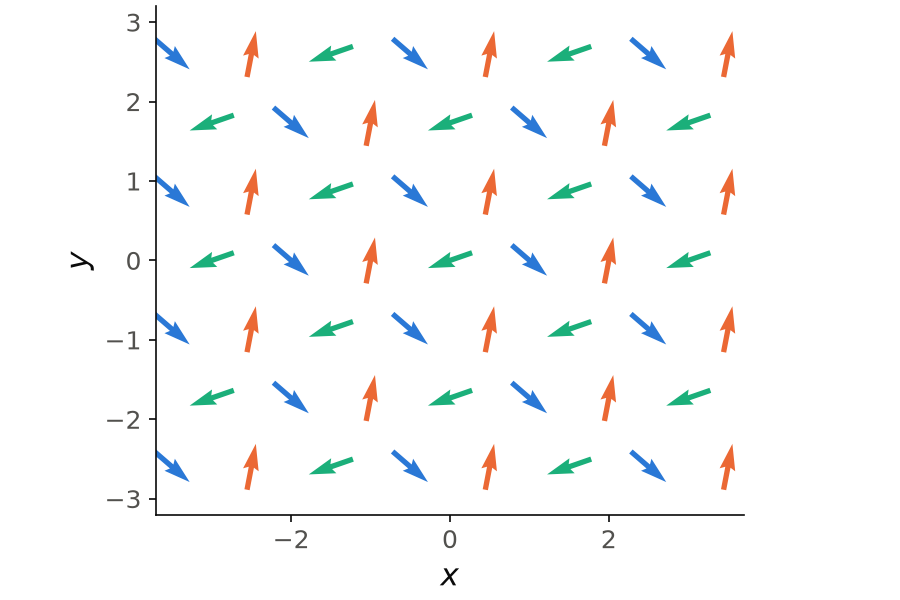
The arrows are the spins, rotated with most_perp_basis() into the frame where they lie in the plane of the figure, and the \(3\times3\) supercell is repeated to fill the window. The three colors are the three sublattices. The spins of each sublattice are parallel, and the three directions are at 120 degrees from each other, so every triangle has one spin of each color. The minimum energy printed by the run is \(-27\) for the 9 sites, so \(-3J\) per site, the value found above. The common direction of the spins is random, since the energy does not depend on it; the script fixes the random seed, so it is the same in every run.

Code of this figure (documentation/figures/classicalspins_120.py)

import numpy as np
import style
from pyqula import geometry
from pyqula import classicalspin
from pyqula.classicalspintk.align import most_perp_basis
np.random.seed(1) # fixed seed, so that every run gives the same figure

g = geometry.triangular_lattice() # geometrically frustrated lattice
g = g.get_supercell(3)

sm = classicalspin.SpinModel(g) # classical spin model on this geometry
sm.add_heisenberg(Jij=[1.0]) # first-neighbor antiferromagnetic exchange
sm.minimize_energy(tries=10) # multistart local minimization

mx,my,mz = sm.get_magnetization() # per-site magnetization components
m = most_perp_basis(np.array([mx,my,mz]).T) # rotate the spins into the xy plane

def draw(ax, c):
    phi = np.arctan2(m[:,1], m[:,0]) # in-plane angle of each spin
    sub = np.round((phi - phi[0])/(2*np.pi/3)).astype(int) % 3 # its sublattice
    for i in range(-2,3): # draw copies of the supercell
        for j in range(-2,3):
            r = g.r + i*g.a1 + j*g.a2
            for s in range(3):
                k = (sub == s) & (abs(r[:,0]) < 3.6) & (abs(r[:,1]) < 3.0)
                ax.quiver(r[k,0], r[k,1], m[k,0], m[k,1], color=c.series[s],
                          pivot="middle", scale=1.7, scale_units="xy", width=0.009)
    ax.set_aspect("equal")
    ax.set_xlim(-3.7, 3.7) ; ax.set_ylim(-3.2, 3.2)
    ax.set_xlabel("$x$") ; ax.set_ylabel("$y$")

style.save(draw, "classicalspins_120")

Other couplings

• add_heisenberg(Jij=[J1,J2,...]): isotropic exchange to first, second, third neighbors, as in g.get_hamiltonian(tij=...).
• add_heisenberg(..., Jm=[Jx,Jy,Jz]): anisotropic diagonal exchange, for example an XXZ model.
• add_field(v): the same field \(\vec b\) on every site.
• classicalspin.generating_functions(name=...): ready-made couplings between two positions, "Linear" (dipolar, \(1/r^3\)), "RKKYTI" (RKKY on the surface of a topological insulator), "ZZ" and "XYZ" (Ising and anisotropic diagonal), "DM" (Dzyaloshinskii-Moriya).
• add_tensor(fun): add the coupling fun between the sites of the unit cell.
• add_tensor_2d(fun,ncells=...,vspiral=...): the same, summed over the periodic images, with an optional rotation of the coupling from image to image to describe a spin spiral with wavevector vspiral.
• get_local_energy(): the energy of each site, for a map of a skyrmion or a domain wall.
• classicalspintk.align.most_perp_basis(): rotates a texture into the frame where it is mostly in-plane, the frame to draw it with arrows.

See examples/classicalspin/ for runnable scripts, among them the 120-degree state drawn with arrows and its local energy (perpendicular/), and a ladder with a modulated exchange whose texture is then used in a quantum Hamiltonian (modulated_ladder/). See jupyter-notebooks/functionalities/classical_spin_models_monte_carlo/01_classical_heisenberg.ipynb and 02_magnetization_textures.ipynb in the same folder for executed notebooks.