Quantum geometry and Berry curvature

The Berry curvature is only one part of the geometry of the Bloch states. In this page we compute the full quantum geometric tensor, whose other part is the quantum metric, and then we resolve the Berry curvature in energy and in real space.

Quantum geometric tensor

The quantum geometric tensor is computed with h.get_quantum_geometric_tensor(). Its antisymmetric part is the Berry curvature. Its symmetric part is the quantum metric, which measures the distance between neighboring Bloch states. In a flat band the metric is the important quantity: it says how spread the states are, and it controls, for example, the superfluid weight of a flat-band superconductor (see Superconductivity).

For a chosen subspace \(S\) of bands, for example the occupied bands, the tensor is

\[ Q_{ij}^{mn}(\mathbf k) = \sum_{l \notin S} \frac{\langle u_m|\partial_{k_i} H|u_l\rangle \langle u_l|\partial_{k_j} H|u_n\rangle} {(E_m-E_l)(E_n-E_l)}, \qquad m,n \in S , \]

where \(m\) and \(n\) are bands of the subspace, \(l\) runs over the bands outside it, \(|u\rangle\) are the Bloch states and \(E\) their energies. The quantum metric and the Berry curvature are

\[ g_{ij} = \mathrm{Re}\,\sum_{m\in S} Q_{ij}^{mm}, \qquad \Omega_{ij} = -2\,\mathrm{Im}\,\sum_{m\in S} Q_{ij}^{mm} . \]

Only states outside \(S\) appear in the energy denominators. So the formula is well defined when \(S\) contains degenerate bands: a spin-degenerate pair, the Kramers pairs of a model with inversion and time-reversal symmetry, or several orbitals that meet at a high-symmetry point. The only case that fails is a degeneracy between \(S\) and a band outside it, and then the call raises a ValueError. The derivative \(\partial_{k_i} H\) is computed analytically from the hoppings, without finite differences.

The tensor of each pair of bands

The individual entries \(Q_{ij}^{mn}\) are not physical. A rotation of the states of \(S\) among themselves, which is a free choice inside a degenerate multiplet, also rotates the tensor. Only its trace and its invariants are physical. For this reason non_abelian=True returns the tensor in the orbital basis,

\[ Q_{ij}(\mathbf k) = \sum_{m,n\in S} |u_m\rangle\, Q_{ij}^{mn}\, \langle u_n| = P\,\partial_{k_i}P\,\partial_{k_j}P\,P , \]

where \(P\) is the projector on \(S\). This depends only on the subspace, not on the basis chosen inside it. Its trace is the tensor above, and in any basis \(|v_m\rangle\) of \(S\) the tensor of each pair of bands is \(\langle v_m|Q_{ij}|v_n\rangle\).

Coordinates

The momenta are in reduced coordinates, \(\mathbf k = \sum_i k_i \mathbf b_i\), with \(\mathbf b_i\) the reciprocal lattice vectors and \(k_i\) of period 1, as everywhere in pyqula. The tensor in Cartesian momenta, the one to compare with a continuum calculation, is \(J Q J^T\) with \(J_{\alpha i} = (\mathbf a_i)_\alpha/2\pi\). coordinates="cartesian" returns it, as a \(3\times3\) tensor in \(x\), \(y\) and \(z\). Only this tensor has the symmetry of the crystal, because the reciprocal lattice vectors are in general not orthogonal. For example, on the honeycomb lattice the trace of the reduced metric is not \(g_{xx}+g_{yy}\), and it is different at the three M points.

Positions of the orbitals

The band structure does not depend on where the orbitals are inside the unit cell, but the Bloch states do, and so does their geometry. We can write the Bloch Hamiltonian with the phase \(e^{i\mathbf k\cdot\mathbf R}\) of the lattice vector only, as if every orbital were at the origin of its cell, or with the full bond vector, \(e^{i\mathbf k\cdot(\mathbf R+\mathbf r_j-\mathbf r_i)}\). The two choices give the same bands and the same Chern number, but a different Berry curvature and quantum metric at each \(\mathbf k\), and a different Brillouin-zone integral of the metric. Only the second one is the geometry of the crystal. It respects the point group: on the honeycomb lattice with a Haldane flux and a sublattice imbalance, the Berry curvature is the same at three \(\mathbf k\)-points related by a \(C_3\) rotation, while with the first choice it even changes sign between them. And it does not depend on the choice of unit cell: the Brillouin-zone average of \(\mathrm{Tr}\,g\), which is the gauge-invariant spread of the Wannier functions of the subspace, doubles exactly when the cell is doubled.

• gauge="atomic" (default): every orbital at its position in the geometry.
• gauge="lattice": every orbital at the origin of its cell. This is the convention of part of the work on flat-band superconductivity, and the one to use to reproduce numbers from it. The dependence on the orbital positions is discussed by Simon and Rudner, Phys. Rev. B 102, 165148.

Code

from pyqula import geometry
from pyqula import topology
g = geometry.honeycomb_lattice() # create honeycomb lattice
h = g.get_hamiltonian() # create hamiltonian of the system (spinful by default)
h.add_haldane(0.2) # Add Haldane coupling
h.shift_fermi(0.3) # put the Fermi level safely mid-gap (gap is [-0.9,0.9])

Q = h.get_quantum_geometric_tensor(k=[0.1,0.2,0.],occ_idxs=[0,1]) # at a k-point
g_metric = h.get_quantum_metric(k=[0.1,0.2,0.],occ_idxs=[0,1]) # quantum metric only

# non-Abelian tensor of the two occupied bands, in the orbital basis
Qna = topology.quantum_geometric_tensor(h,k=[0.1,0.2,0.],occ_idxs=[0,1],
        non_abelian=True)

# along a k-path, and integrated over the BZ: the integral of the Berry
# curvature part reproduces h.get_chern()
inds,gpath,omegapath = topology.quantum_geometric_tensor_path(h,occ_idxs=[0,1])
C = topology.chern_from_qgt(h,nk=20,occ_idxs=[0,1])

In two dimensions Q is a complex \(2\times2\) array, one entry per pair of directions, and the metric is its real part. With non_abelian=True it is a \(2\times2\times4\times4\) array: one \(4\times4\) matrix in the spin-orbital basis for each pair of directions. There is no spin-orbit coupling here, so this matrix is block diagonal in spin, and the trace over the spin-up orbitals is the contribution of the spin-up electrons. Along the k-path the function returns the position along the path, and the metric and the curvature at each point, one \(2\times2\) tensor per k-point. The integral of the curvature over the Brillouin zone gives the Chern number, here \(C=2\) for the two spin-degenerate occupied bands, the same as h.get_chern().

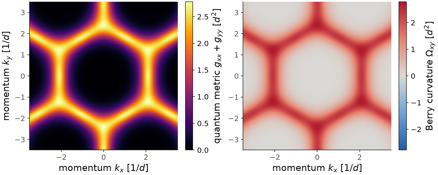
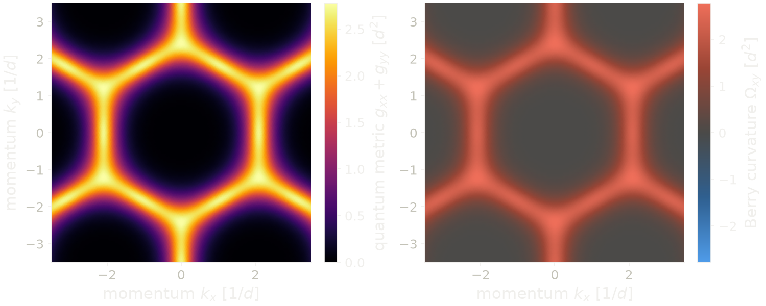
The figure shows the same tensor on a \(60\times60\) k-mesh, from topology.quantum_geometric_tensor_mesh(h,nk=60,occ_idxs=[0,1],coordinates="cartesian"). We use Cartesian momenta, so that the maps have the hexagonal symmetry of the crystal. Momenta are in units of \(1/d\), with \(d\) the first-neighbor distance, and the tensor is in units of \(d^2\). The trace of the metric, \(g_{xx}+g_{yy}\), and the Berry curvature are both largest at the K and K' points, the corners of the hexagons, with \(2.78\), and both are zero at \(\Gamma\). The curvature is positive everywhere. At every k-point the trace of the metric is larger than or equal to the curvature, by at most \(0.32\), and the two are equal at K and K'. Averaged over the Brillouin zone, the trace of the metric is \(0.89\) and the curvature \(0.83\).

Code of this figure (documentation/figures/geometry_qgt.py)

import numpy as np
import style
from pyqula import geometry
from pyqula import topology
g = geometry.honeycomb_lattice() # create honeycomb lattice
h = g.get_hamiltonian() # create hamiltonian of the system (spinful by default)
h.add_haldane(0.2) # Add Haldane coupling
h.shift_fermi(0.3) # put the Fermi level safely mid-gap (gap is [-0.9,0.9])

Q = h.get_quantum_geometric_tensor(k=[0.1,0.2,0.],occ_idxs=[0,1]) # at a k-point
g_metric = h.get_quantum_metric(k=[0.1,0.2,0.],occ_idxs=[0,1]) # quantum metric only

# non-Abelian tensor of the two occupied bands, in the orbital basis
Qna = topology.quantum_geometric_tensor(h,k=[0.1,0.2,0.],occ_idxs=[0,1],
        non_abelian=True)

# along a k-path, and integrated over the BZ: the integral of the Berry
# curvature part reproduces h.get_chern()
inds,gpath,omegapath = topology.quantum_geometric_tensor_path(h,occ_idxs=[0,1])
C = topology.chern_from_qgt(h,nk=20,occ_idxs=[0,1])

# the tensor on a k-mesh, in Cartesian momenta
ks,Qk = topology.quantum_geometric_tensor_mesh(h,nk=60,occ_idxs=[0,1],
        coordinates="cartesian")
trg = (Qk[:,0,0]+Qk[:,1,1]).real # trace of the quantum metric, g_xx+g_yy
omega = -2*Qk[:,0,1].imag # Berry curvature
ks = [ks+[i,j,0] for i in range(-2,2) for j in range(-2,2)] # 16 copies of the BZ
kxy = 2*np.pi*np.array([k[:,0:1]*g.b1+k[:,1:2]*g.b2 for k in ks]).reshape(-1,3) # Cartesian
trg,omega = np.tile(trg,16),np.tile(omega,16)

def draw(ax, c):
    m = np.max(np.abs(omega))
    p0 = ax[0].tripcolor(kxy[:,0], kxy[:,1], trg, cmap=c.cmap, shading="gouraud")
    p1 = ax[1].tripcolor(kxy[:,0], kxy[:,1], omega, cmap=c.diverging,
                         vmin=-m, vmax=m, shading="gouraud")
    style.colorbar(p0, ax[0], r"quantum metric $g_{xx}+g_{yy}$ [$d^2$]")
    style.colorbar(p1, ax[1], r"Berry curvature $\Omega_{xy}$ [$d^2$]")
    for axi in ax:
        axi.set_xlim(-3.5, 3.5)
        axi.set_ylim(-3.5, 3.5)
        axi.set_aspect("equal")
        axi.set_xlabel(r"momentum $k_x$ [$1/d$]")
    ax[0].set_ylabel(r"momentum $k_y$ [$1/d$]")

style.save(draw, "geometry_qgt", npanels=2)

• occ_idxs: the indices of the bands in \(S\). By default, the bands with \(E<0\), as in h.get_chern(), so it follows h.shift_fermi().
• k: the k-point, in reduced coordinates.
• non_abelian, coordinates, gauge: as explained above.

The same functions work in one and three dimensions, where the tensor has one and nine components, and topology.quantum_geometric_tensor_mesh(h,nk=...) returns it on a uniform k-mesh.

See examples/2d/quantum_geometric_tensor/main.py for the spin-resolved tensor above, examples/2d/quantum_geometry/main.py for the Berry curvature and the metric of the occupied bands along a k-path, and jupyter-notebooks/functionalities/topological_characterization/06_quantum_geometric_tensor.ipynb.

Berry curvature density in energy

The Chern number is one integer for all the occupied bands. To see from which energies it comes, we use topology.chern_density(). The Berry curvature of the occupied states is written as an integral over energy,

\[ \Omega (\mathbf k) = \int_{-\infty}^{\epsilon_F} \Xi (\mathbf k,\omega)\, d\omega , \]

where \(\Xi (\mathbf k,\omega)\) is the energy-resolved Berry curvature: how much curvature the states at energy \(\omega\) carry. It is built from the Green's function with a broadening delta. topology.chern_density() integrates \(\Xi(\mathbf k,\omega)\) over the Brillouin zone at a set of energies, and also returns its cumulative integral in energy.

from pyqula import geometry
from pyqula import topology
import numpy as np
g = geometry.honeycomb_lattice() # create honeycomb lattice
h = g.get_hamiltonian() # create hamiltonian of the system
h.add_haldane(0.05) # Add Haldane coupling
es = np.arange(-3.5,3.5+1e-9,0.05) # from below the band to above it
(es,cs,csi,cex) = topology.chern_density(h,nk=12,delta=0.1,es=es,exact_at=[0.])

es are the energies, cs the Berry curvature density at each energy, and csi its cumulative integral, which starts at the first energy of es. cex is the cumulative integral without broadening at the energies of exact_at, explained below. Inside the gap csi has a plateau, and when the integral goes over all the bands it comes back to zero, because the Berry curvatures of all the bands of a Hamiltonian add up to zero. The normalization is the one of h.get_chern(), but the plateau of csi is the Chern number only in a limit that is expensive to reach. The snippet takes about 20 seconds, and its plateau at zero energy is \(1.63\), not \(C=2\). Four things decide how close the plateau is to the Chern number, and the snippet is chosen to respect the first three; the fourth is the broadening, which exact_at removes.

• The integral starts at the first energy of es, so es must start below the bottom of the band, here \(-3\). A window that starts at \(-1\) misses the curvature of the lower states: with es from \(-1\) to \(1\), delta=0.02 and dk=0.02, the plateau is \(3.97\) at nk=10, \(3.18\) at nk=20 and \(2.91\) at nk=40, and none of these is the Chern number.
• The energy step must be at most delta/2, otherwise the peak of each state is not resolved. At delta=0.05 and nk=12 a step of delta/4 changes the plateau by \(10^{-3}\), but a step of delta changes it by \(0.12\). The snippet has a step of \(0.05\) for delta=0.1.
• The derivatives in momentum are finite differences with a step dk, in units of the reciprocal lattice vectors. Over dk the bands must move by much less than delta, so the default is dk=delta/25. A fixed step is too large at a small delta: at delta=0.05 and nk=20 the plateau is \(1.62\) with dk=0.02, \(1.69\) with dk=0.005 and the same with dk=0.001.
• The broadening delta spreads the curvature of the states above the gap into the gap. With es from \(-3.5\) to \(0\), a step of delta/2 or smaller and a small enough dk, the plateau at zero energy is \(1.70\) for delta=0.05 (\(1.69\), \(1.71\) and \(1.70\) at nk=20, \(24\) and \(40\)), \(1.86\) for delta=0.02 at nk=20, and between \(1.92\) and \(1.98\) for delta=0.01 at nk=20, \(21\) and \(30\). It goes up towards \(C=2\) as delta goes down, slowly, and a smaller delta needs a finer nk, a finer energy step and a smaller dk.

The broadening can be removed exactly at energies inside a gap. The cumulative integral is an integral of an analytic function of the complex energy \(\omega+i\delta\), along the line at height delta. Inside a gap that function is smooth down to the real axis, so we can close the path with a vertical segment from \(\omega+i\delta\) down to \(\omega\), and another one at the first energy of es, below the band. The result is the integral with no broadening at all, meaning that it does not depend on delta. This is what exact_at does, for the energies it lists. In the snippet cex is \(2.56\), and \(2.58\) with delta=0.05, while csi moves from \(1.63\) to \(2.08\). What is left is the k-mesh, since the curvature is a sum over the k-points of the mesh: cex is \(2.01\) at nk=24 and \(1.99\) at nk=36, the Chern number. Each energy of exact_at costs about as much as 9 energies of es, and inside a band the vertical segment is not smooth, so the result there has no meaning.

So read csi as a profile in energy, and cex as the number. The density also needs a fine enough nk for its delta, otherwise it shows spurious peaks near k-points where bands come close.

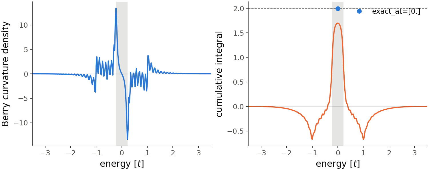
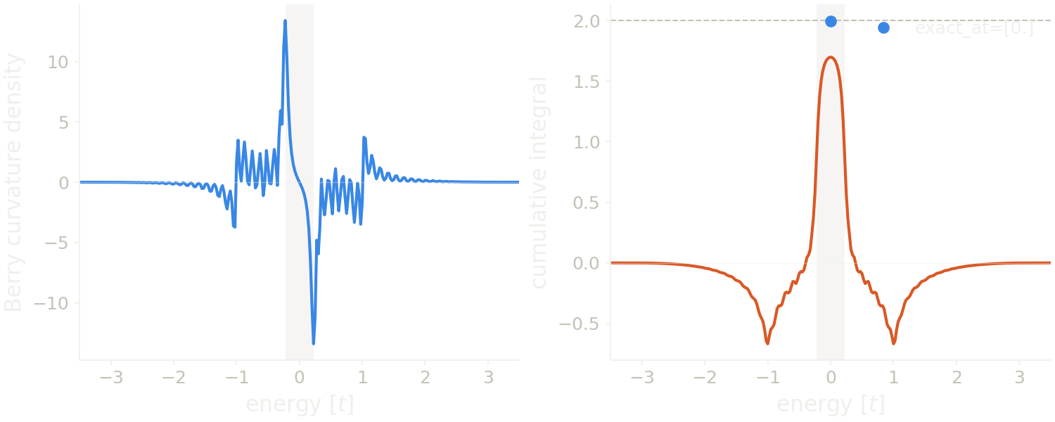
The figure shows cs on the left and csi on the right, for the snippet with a smaller broadening and a finer mesh: es from \(-3.5\) to \(3.5\) with a step of delta/2, delta=0.05, nk=48 and exact_at=[0.]. This takes about 15 minutes. A multiple of 3 for nk puts the K points on the mesh, so the band edges are where they should be. The gray band is the bulk gap, from \(-0.225\) to \(0.225\). The density has its two largest peaks at the band edges, of opposite sign, and the cumulative integral has its plateau in the gap, \(1.70\) at zero energy, the same as at nk=24 within \(0.01\). The dashed line is the Chern number, \(C=2\): the plateau is below it by \(0.30\), the curvature that delta=0.05 moves into the gap. The dot is cex at zero energy, \(1.998\), the same integral without the broadening. The density is odd in energy, so the cumulative integral comes back to zero at the end of the window. Away from the gap the density still oscillates. Each oscillation is a group of k-points of the mesh, which delta=0.05 does not merge; from the energy step between neighboring k-points we estimate that a smooth density at this delta needs nk above about \(100\). The integral averages the oscillations out, so the plateau is converged while the density is not.

Code of this figure (documentation/figures/geometry_chern_density.py)

import style
from pyqula import geometry
from pyqula import topology
import numpy as np
g = geometry.honeycomb_lattice() # create honeycomb lattice
h = g.get_hamiltonian() # create hamiltonian of the system
h.add_haldane(0.05) # Add Haldane coupling
# the snippet of the page, converged: the energies start below the bottom of
# the band, with a step of delta/2, the k-mesh contains the K points (nk is a
# multiple of 3), and the finite-difference step dk is delta/25, the default
delta = 0.05
es = np.arange(-3.5,3.5+1e-9,delta/2)
(es,cs,csi,cex) = topology.chern_density(h,nk=48,es=es,delta=delta,
                                         exact_at=[0.]) # without broadening at E=0
print("plateau at zero energy:",np.interp(0.,es,csi),"exact:",cex[0])
(k,e) = h.get_bands() # bands, to mark the gap
gap = np.min(e[e>0]) # the gap is from -gap to gap

def draw(ax, c):
    ax[0].plot(es, cs, color=c.blue)
    ax[1].plot(es, csi, color=c.orange)
    ax[1].axhline(2, color=c.ink2, lw=1.0, ls="--") # the Chern number
    ax[1].plot([0.], cex, "o", color=c.blue, ms=7, label="exact_at=[0.]")
    ax[1].legend(loc="upper right")
    ax[0].set_ylabel("Berry curvature density")
    ax[1].set_ylabel("cumulative integral")
    for axi in ax:
        axi.axvspan(-gap, gap, color=c.ink2, alpha=0.15, lw=0) # the bulk gap
        axi.axhline(0, color=c.ink, lw=0.6, alpha=0.4)
        axi.set_xlabel("energy [$t$]")
        axi.set_xlim(-3.5, 3.5)

style.save(draw, "geometry_chern_density", npanels=2)

• nk: number of k-points per direction of the mesh.
• es: energies at which the density is computed.
• delta: broadening of the Green's function.
• exact_at=None: energies inside gaps where the cumulative integral is also returned without broadening, as a fourth array.
• nodes=8: number of points of the vertical segments of exact_at.
• dk: step of the finite differences in momentum, in units of the reciprocal lattice vectors, delta/25 by default.
• operator: weight the curvature with an operator, as in h.get_chern().
• write: if True, also write CHERN_DENSITY.OUT and CHERN_DENSITY_INTEGRATED.OUT.

The map of \(\Xi(\mathbf k,\omega)\) over the Brillouin zone at one energy is given by topology.dOmega_dE_kmap(h,nk=40,e=0.), which writes it to BERRY_DENSITY_KMAP.OUT. It covers the same window of whole Brillouin zones as h.get_berry_curvature(), so the mean of the map divided by \(2\pi\) is the value of cs at that energy, for the same delta and dk. See examples/2d/berry_density/main.py, examples/2d/chern_density/main.py and examples/2d/berry_density_kmap/main.py, and jupyter-notebooks/functionalities/topological_characterization/03_frequency_resolved_topological_density.ipynb.

Berry curvature density in real space

A Chern number needs a Brillouin zone. The Berry curvature can also be resolved in real space, to see where in the sample the topological flux is. This also works for an island, a disordered sample, or a supercell too large for a k-mesh. It is computed with topology.real_space_chern(). The idea is

\[ \Omega (\mathbf k) = \int \Gamma (\mathbf k,\mathbf r)\, d^2 \mathbf r , \]

where \(\Gamma (\mathbf k,\mathbf r)\) is the Berry curvature resolved in position. In practice, for a finite system, pyqula computes a local Chern marker of the Bianco-Resta type,

\[ C(\mathbf r) = \frac{2\pi}{A_{\mathbf r}}\, \mathrm{Im}\,\langle \mathbf r|\, [PxP,\, PyP] \,|\mathbf r\rangle , \]

with \(P\) the projector on the occupied states, \(x\) and \(y\) the position operators, the diagonal element summed over the orbitals of the site \(\mathbf r\), and \(A_{\mathbf r}\) the area of the site. The occupied states are those below zero energy, so a Hamiltonian whose gap is not at zero must be shifted first, for example with h.set_filling(0.5). Deep in the bulk this local quantity is the Chern number.

from pyqula import islands
from pyqula import topology
g = islands.get_geometry(name="honeycomb",n=8,nedges=3) # a honeycomb island
h = g.get_hamiltonian() # create hamiltonian of the system
h.add_haldane(0.05) # Add Haldane coupling
(r,c) = topology.real_space_chern(h) # spatially-resolved Berry curvature

r are the positions of the sites and c the local marker at each site. The call also writes REAL_SPACE_CHERN.OUT, one value per site, to plot as a map over the island. The Hamiltonian must be finite; a periodic one raises a ValueError. For a periodic system, build a large supercell and make it finite first. How to read the marker, and how to get the Chern number from it, is explained in Topology in real space.

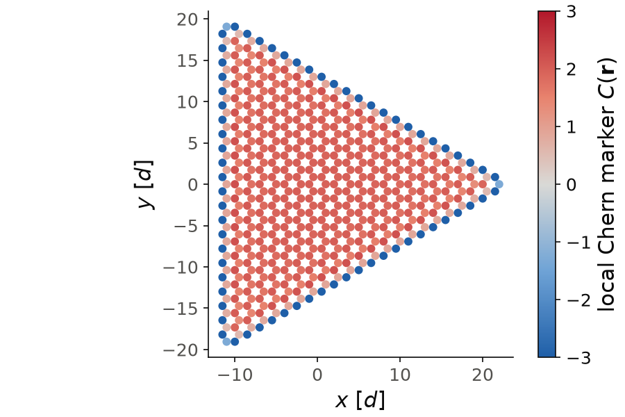
The figure shows c at each site of the island of the snippet, a triangle of \(573\) sites, with the color scale cut at \(\pm3\). Within a distance of \(8\) from the center, the marker is between \(1.75\) and \(2.02\), close to \(C=2\). The sites of the outermost row are strongly negative, down to \(-17.6\), and they compensate the bulk.

Code of this figure (documentation/figures/geometry_realspace.py)

import numpy as np
import style
from pyqula import islands
from pyqula import topology
g = islands.get_geometry(name="honeycomb",n=8,nedges=3) # a honeycomb island
h = g.get_hamiltonian() # create hamiltonian of the system
h.add_haldane(0.05) # Add Haldane coupling
(r,c) = topology.real_space_chern(h) # spatially-resolved Berry curvature
r = np.array(r) # positions of the sites

def draw(ax, cl):
    sc = ax.scatter(r[:,0], r[:,1], c=c, s=22, cmap=cl.diverging, vmin=-3, vmax=3)
    style.colorbar(sc, ax, r"local Chern marker $C(\mathbf{r})$")
    ax.set_aspect("equal")
    ax.set_xlabel("$x$ [$d$]")
    ax.set_ylabel("$y$ [$d$]")

style.save(draw, "geometry_realspace")

See examples/0d/real_space_chern/main.py and jupyter-notebooks/functionalities/topological_characterization/04_spatially_resolved_topological_flux.ipynb.