Entanglement

In this page we compute the entanglement entropy of a region of a ground state, with h.get_entanglement_entropy(), and its entanglement spectrum, with h.get_entanglement_spectrum().

Entanglement entropy and entanglement spectrum

The ground state of a non-interacting or mean-field Hamiltonian is a Slater determinant. For a Slater determinant, the reduced density matrix of a region \(A\) is the exponential of a single-particle operator, so it is fixed by the correlations inside \(A\) only. We compute the correlation matrix restricted to the region,

\[ C_{ij} = \langle c_i^\dagger c_j\rangle, \qquad i,j \in A , \]

and diagonalize it. Its eigenvalues \(\zeta_n\) are between 0 and 1, and they give

\[ S = -\sum_n \left[ \zeta_n \ln \zeta_n + (1-\zeta_n)\ln(1-\zeta_n)\right], \qquad \xi_n = \ln\frac{1-\zeta_n}{\zeta_n} , \]

the entanglement entropy \(S\) and the single-particle entanglement spectrum \(\xi_n\). An eigenvalue at 0 or 1 is a state fully outside or fully inside the region, and it does not contribute to the entropy. An eigenvalue at \(1/2\), \(\xi_n=0\), is a state shared equally between the region and the rest, and it contributes the most, \(\ln 2\). Only a matrix of the size of the region is diagonalized, never the reduced density matrix itself, so large regions are cheap.

The region is given as a list of site indices, a boolean mask, a function of the position, or a fraction of the cells. Spin, sublattice and Nambu components are orbitals of a site, so a region is always a set of sites. A periodic Hamiltonian is first folded into a ring of nsuper unit cells, so the region \(A\) has two boundaries, not one. Its entropy is then twice the entropy of a single cut. Keep this in mind when comparing with a formula written for one boundary.

The entanglement spectrum as a topological probe

In a two-dimensional system cut along one direction, the momentum \(k_\parallel\) parallel to the cut is still a good quantum number, and \(\xi_n(k_\parallel)\) is the Li-Haldane entanglement spectrum. For a Chern insulator, it has branches that cross \(\xi=0\) inside its gap, \(2|C|\) of them: \(|C|\) chiral modes for each of the two boundaries. This is the same as the edge spectrum of the model. For a trivial insulator, the entanglement spectrum has a gap around \(\xi=0\). This is a calculation of the bulk ground state only: no ribbon and no open boundary is built, and the edge states are read from the bulk.

from pyqula import geometry
g = geometry.honeycomb_lattice() # create a honeycomb lattice
h = g.get_hamiltonian(has_spin=False) # get the Hamiltonian
h.add_haldane(0.1) # Chern insulator, C = 1
print(h.get_chern(nk=20)) # 1.0

# Li-Haldane entanglement spectrum xi_n(k_par) across the BZ
(ks,xis) = h.get_entanglement_spectrum(nsuper=10,nk=101)

# entanglement entropy, per parallel unit cell, averaged over the BZ
print(h.get_entanglement_entropy(nsuper=10,nk=20))

ks are the nk parallel momenta across the Brillouin zone. xis has one row per momentum and one column per orbital of the region, ten here (half of a ring of ten cells, with two sites per cell). If you plot every column against ks, you see the levels of the Chern insulator crossing \(\xi=0\). The same plot for the honeycomb lattice gapped by a sublattice imbalance shows a spectrum that never comes close to zero. The entropy is given per parallel unit cell, averaged over nk momenta, and it counts both boundaries of the region.

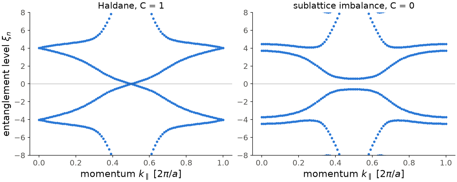
On the left is the spectrum of the snippet. On the right is the same lattice with a sublattice imbalance of \(0.3\) instead of the Haldane coupling, a trivial insulator. In the Chern insulator two levels cross \(\xi=0\) at \(k_\parallel=1/2\), in opposite directions: one for each boundary of the region, so \(2|C|=2\) crossings. In the trivial insulator no level comes closer to zero than \(0.59\). The plot is cut at \(\pm8\); the levels beyond are states almost fully inside or fully outside the region, which do not contribute to the entropy.

Code of this figure (documentation/figures/entanglement_spectrum.py)

import style
from pyqula import geometry
g = geometry.honeycomb_lattice() # create a honeycomb lattice
h = g.get_hamiltonian(has_spin=False) # get the Hamiltonian
h.add_haldane(0.1) # Chern insulator, C = 1
print(h.get_chern(nk=20)) # 1.0

# Li-Haldane entanglement spectrum xi_n(k_par) across the BZ
(ks,xis) = h.get_entanglement_spectrum(nsuper=10,nk=101)

# entanglement entropy, per parallel unit cell, averaged over the BZ
print(h.get_entanglement_entropy(nsuper=10,nk=20))

h0 = g.get_hamiltonian(has_spin=False) # the trivial insulator, for comparison
h0.add_sublattice_imbalance(0.3) # gapped by a sublattice imbalance
(ks0,xis0) = h0.get_entanglement_spectrum(nsuper=10,nk=101)

def draw(ax, c):
    for (axi,k,xi,name) in zip(ax,[ks,ks0],[xis,xis0],["Haldane, C = 1","sublattice imbalance, C = 0"]):
        for col in xi.T: # one level per orbital of the region
            axi.scatter(k, col, s=8, color=c.blue)
        axi.axhline(0, color=c.ink, lw=0.6, alpha=0.4)
        axi.set_ylim(-8, 8)
        axi.set_xlabel(r"momentum $k_\parallel$ [$2\pi/a$]")
        axi.set_title(name)
    ax[0].set_ylabel(r"entanglement level $\xi_n$")

style.save(draw, "entanglement_spectrum", npanels=2)

Keywords:

• region: the region \(A\), in one of the four forms above. None takes half of the system.
• nsuper: number of unit cells of the ring, for a periodic Hamiltonian.
• direction: the lattice direction normal to the cut, by default the last periodic one.
• kpar: a single parallel momentum. With None, a two-dimensional Hamiltonian is swept or averaged over nk momenta.
• nk: number of parallel momenta.
• fermi: the states with \(E<\) fermi are occupied, zero by default.

Remarks

For a Bogoliubov-de Gennes Hamiltonian, the correlation matrix includes the anomalous correlations \(\langle c_i c_j\rangle\), and the doubling of the Nambu basis is divided out. fermi must stay at zero in this case, because the chemical potential is already in the Hamiltonian.

The occupation is taken at zero temperature. A level exactly at the Fermi energy makes the ground state degenerate, and then the entropy depends on which state is chosen, so the call raises an error. On a ring this happens for some values of nsuper, for example for a half-filled chain with nsuper divisible by four. Changing the size of the ring by one solves it.

As a reference, the critical chain gives the conformal field theory result with central charge \(c=1\),

\[ S = \frac{c}{3}\ln\left[\frac{L}{\pi}\sin\frac{\pi l}{L}\right] , \]

for a region of \(l\) cells in a ring of \(L\) cells. A gapped two-dimensional insulator follows the area law instead, the entropy proportional to the length of the boundary.

See examples/1d/entanglement_entropy_chain/main.py (the central charge from a fit of the entropy against the size of the region) and examples/2d/entanglement_spectrum_haldane/main.py (the spectrum of the Haldane model next to the one of a trivial insulator) for scripts that make the plots, and jupyter-notebooks/functionalities/topological_characterization/12_entanglement.ipynb.