Mean-field Hubbard models

So far all our Hamiltonians were single-particle Hamiltonians: every term is bilinear, one creation and one annihilation operator. An interaction between electrons is a quartic term, with four fermion operators, and the problem is then a quantum many-body one. In this page we treat interactions at the mean-field level. The quartic term is replaced by bilinear terms that depend on expectation values in the ground state. These expectation values depend on the Hamiltonian, so the problem is solved self-consistently.

Mean field is an uncontrolled approximation. It does not capture quantum fluctuations, so it overestimates ordering, and in low dimensions it finds order where the exact ground state has none. Still, it is the practical way to describe magnetism, charge order and superconductivity driven by interactions. Everything in this page uses one method, h.get_mean_field_hamiltonian(), which returns a new Hamiltonian with the converged mean-field terms. The original h is not changed.

The collinear Hubbard model

We start with the simplest interaction, a local repulsion in a spinful system, the Hubbard model,

\[ H = \sum_{\langle ij\rangle,s} c^\dagger_{i,s} c_{j,s} + h.c. + U\sum_{i} c^\dagger_{i,\uparrow} c_{i,\uparrow} c^\dagger_{i,\downarrow} c_{i,\downarrow} . \]

The first term is the first-neighbor hopping, and \(U\) is the energy cost of having a spin-up and a spin-down electron on the same site, in units of the hopping. The mean-field approximation replaces the quartic term by all the terms we get by taking the expectation value of two of the four operators. The simplest of them, the collinear (Hartree) terms, are

\[ H_U^{MF} = U\sum_{i} \langle n_{i,\uparrow} \rangle n_{i,\downarrow} + n_{i,\uparrow} \langle n_{i,\downarrow} \rangle , \qquad n_{i,s} = c^\dagger_{i,s} c_{i,s} , \]

where \(\langle\cdot\rangle\) is the expectation value in the ground state. So an electron with spin down feels an onsite energy proportional to the density of spin-up electrons on its site, and the other way around. If the two densities are different, the two spins see different onsite energies: this is an exchange field, and the state is magnetic.

The mean-field Hamiltonian depends on the ground state, and the ground state depends on the mean-field Hamiltonian. We solve this by iteration:

\[ |GS_0\rangle \rightarrow H^{MF}_0 \rightarrow |GS_1\rangle \rightarrow H^{MF}_1 \rightarrow |GS_2\rangle \rightarrow \cdots \]

We start from an initial guess \(|GS_0\rangle\), compute \(H^{MF}_0\), diagonalize it to get a new ground state \(|GS_1\rangle\), and so on. The loop stops when two successive mean fields differ by less than maxerror. Two things matter in practice:

• The result can depend on the initial guess. If the energy has several local minima, different guesses can converge to different states. Try several guesses, and compare the total energies.
• The new mean field is mixed with the old one at each step. Close to a phase transition the loop can converge slowly or oscillate.

As an example, we take a square lattice, a \(2\times2\) supercell, and a repulsive \(U\) at half filling. The ground state is an antiferromagnetic Neel state with a gap:

from pyqula import geometry
g = geometry.square_lattice() # geometry of a square lattice
g = g.get_supercell([2,2]) # generate a 2x2 supercell
h = g.get_hamiltonian() # create hamiltonian of the system
h = h.get_mean_field_hamiltonian(U=2.0,filling=0.5,
                            mf="random") # perform SCF
(k,e) = h.get_bands() # calculate band structure
m = h.get_magnetization() # get the magnetization

Without interactions the half-filled square lattice is a metal. With \(U=2\) the band structure has a gap at zero energy of about \(0.8\). The magnetization m has one vector per site. The vectors have the same length, about \(0.38\), and opposite sign on the two sublattices. Their direction is set by the random initial guess, because the Hamiltonian has spin rotation symmetry and nothing selects a direction. We need the supercell because a Neel state has two different sites, and a cell with one site can only hold a ferromagnet. A larger \(U\) gives larger moments and a larger gap. For large \(U\) the gap grows linearly with \(U\), with one localized electron per site.

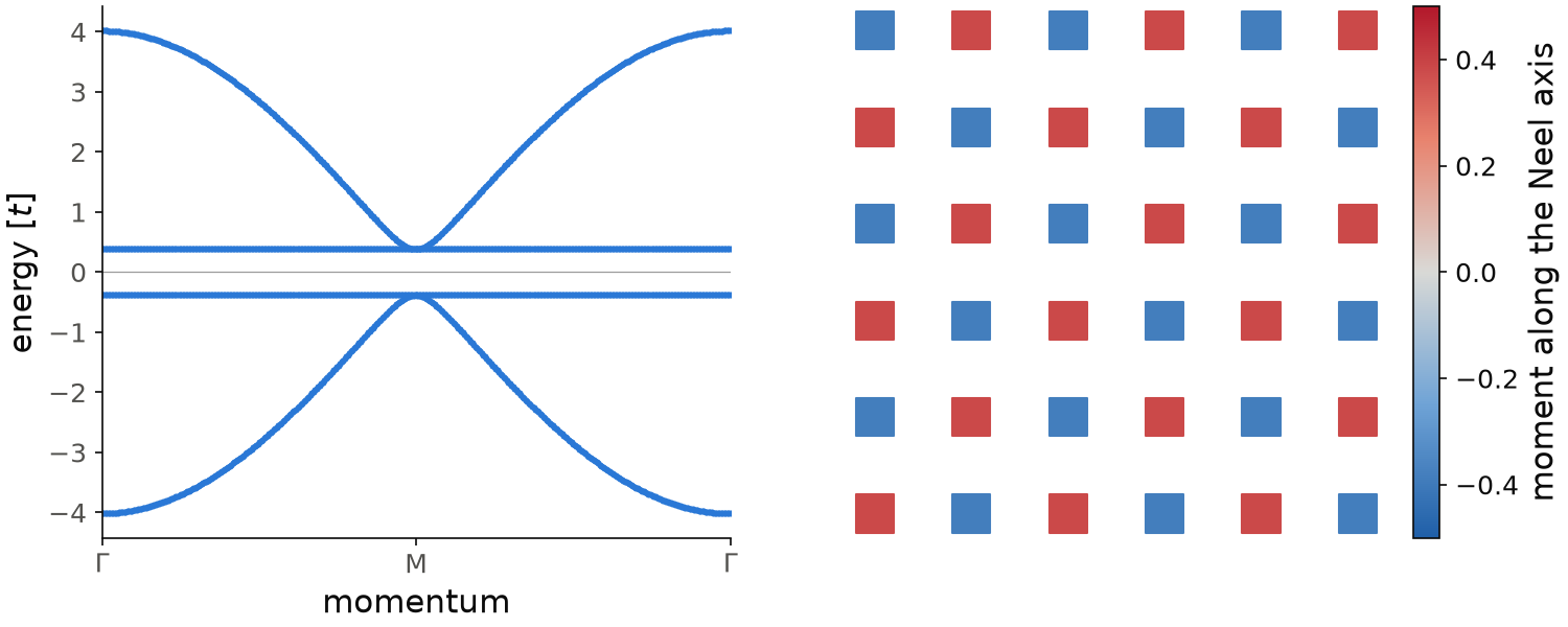
The script fixes the random seed, so that the figure is reproducible. On the left, the band structure has a gap of \(0.77\) at zero energy. The exchange field on each site is \(Um/2=0.38\), with \(m=0.38\) the moment, and the gap is twice this field. The two flat bands at \(\pm0.38\) are states of the k-path that lie on the Fermi surface of the non-interacting model. On the right, the \(2\times2\) cell is repeated three times in each direction, and each site is colored by its moment along the moment of the first site. The moments are \(\pm0.38\), red on one sublattice and blue on the other. This checkerboard is the Neel state, which neutron diffraction sees as a magnetic Bragg peak at \((\pi,\pi)\).

Code of this figure (documentation/figures/meanfield_collinear.py)

import numpy as np
import style
from pyqula import geometry
np.random.seed(0) # fix the random guess, so that the figure is reproducible
g = geometry.square_lattice() # geometry of a square lattice
g = g.get_supercell([2,2]) # generate a 2x2 supercell
h = g.get_hamiltonian() # create hamiltonian of the system
h = h.get_mean_field_hamiltonian(U=2.0,filling=0.5,
                            mf="random") # perform SCF
(k,e) = h.get_bands() # calculate band structure
m = h.get_magnetization() # get the magnetization
ms = m @ m[0]/np.linalg.norm(m[0]) # moment of each site along the one of site 0
r = np.array([ri + i*g.a1 + j*g.a2 for i in range(3) for j in range(3) for ri in g.r])

def draw(axs, c):
    axs[0].scatter(k, e, s=3, color=c.blue)
    axs[0].axhline(0, color=c.ink, lw=0.6, alpha=0.4)
    n = k.max() # the path goes Gamma-M-Gamma
    axs[0].set_xticks([0, n/2, n], [r"$\Gamma$", "M", r"$\Gamma$"])
    axs[0].set_xlim(0, n)
    axs[0].set_xlabel("momentum")
    axs[0].set_ylabel("energy [$t$]")
    sc = axs[1].scatter(r[:,0], r[:,1], c=np.tile(ms, 9), s=300, marker="s",
                        cmap=c.diverging, vmin=-0.5, vmax=0.5)
    axs[1].set_aspect("equal")
    axs[1].axis("off")
    style.colorbar(sc, axs[1], "moment along the Neel axis")

style.save(draw, "meanfield_collinear", npanels=2)
print("moments", ms)
print("gap", e[e>0].min()-e[e<0].max())

The main keywords are:

• U: the Hubbard interaction, a number or one value per site.
• filling: the filling, kept fixed at every iteration (see the filling section of Building a Hamiltonian).
• mf: the initial guess. A name such as "random", "ferro", "antiferro" or "swave", or a Hamiltonian whose mean-field terms are used as the starting point.
• nk: the number of k-points per direction used to compute the expectation values. A metal needs more k-points than an insulator.
• maxerror, mix: the convergence tolerance and the mixing.

If the loop does not converge, the method raises an error instead of returning a Hamiltonian. The page Exchange interactions discusses this case and the parameters that control it.

See examples/2d/hubbard_honeycomb/main.py for the gap as a function of \(U\) on the honeycomb lattice. There the density of states vanishes at the Dirac point, so a small \(U\) does nothing, and the gap opens only above a critical interaction, around \(U\approx 2.2\) at the mean-field level. The notebook jupyter-notebooks/functionalities/interacting_mean_field_hamiltonians/02_collinear_noncollinear.ipynb shows the executed version.

Non-collinear Hubbard model

The collinear terms above only allow a magnetization along one axis. With frustration, an external field or spin-orbit coupling, the magnetization can point in any direction, and change direction from site to site. To describe this, the mean field also includes the spin-flip (Fock) term

\[ H_U^{ncMF} = - U\sum_{i} \langle c^\dagger_{i,\downarrow} c_{i,\uparrow} \rangle c^\dagger_{i,\uparrow} c_{i,\downarrow} + h.c., \]

set by the in-plane magnetization of each site. With this term the mean-field Hubbard Hamiltonian has the full SO(3) spin rotation symmetry of the Hubbard model. pyqula always includes it. This is also why in the previous example the direction of the Neel moments was free.

We now take the same square lattice and add a Zeeman field along \(z\). The Zeeman energy competes with the antiferromagnetic order, and the result is a canted state:

from pyqula import geometry
g = geometry.square_lattice() # geometry of a square lattice
g = g.get_supercell([2,2]) # generate a 2x2 supercell
h = g.get_hamiltonian() # create hamiltonian of the system
h.add_zeeman([0.,0.,0.1]) # add out-of-plane Zeeman field
h = h.get_mean_field_hamiltonian(U=2.0,filling=0.5,
                                  mf="random") # perform SCF
(k,e,c) = h.get_bands(operator="sz") # calculate band structure
m = h.get_magnetization() # get the magnetization

The magnetization now has two parts. The antiferromagnetic part alternates between the sublattices and lies in the plane perpendicular to the field. The uniform part is the same on every site, and it points opposite to the vector given to h.add_zeeman(), because the Zeeman term is \(+\vec B\cdot\vec\sigma\) (see Building a Hamiltonian). The moments cant out of the plane instead of flipping, as an antiferromagnet does in a field that is weak compared to its exchange, and a larger field cants them more. The third array c returned by h.get_bands(operator="sz") is the spin projection \(\langle S_z\rangle\) of each state, so the bands can be colored by it.

From a random guess this loop does not always converge. In 2 of 40 random seeds it stops after maxite iterations and raises an error. For both of them a larger mixing, mix=0.5, or more iterations, maxite=5000, gives a converged state. Calling np.random.seed() before the calculation makes a run reproducible.

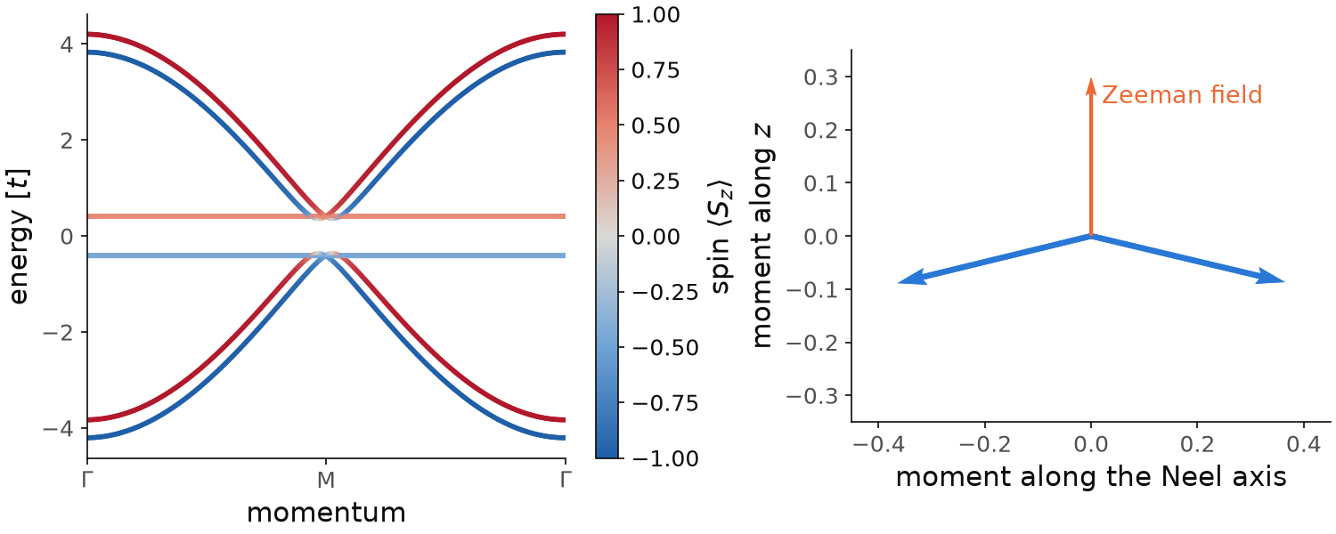
The script fixes the random seed, so that the figure is reproducible. On the left, each band has a spin-up copy, higher in energy, and a spin-down copy, split by the Zeeman field. On the right are the moments of the four sites, in the plane of the Neel axis and of \(z\). The antiferromagnetic part is \(0.36\), in the plane. The uniform part is \(-0.09\) on every site: it points along \(-z\), opposite to the vector given to h.add_zeeman(), because the term is \(+\vec B\cdot\vec\sigma\) (see Building a Hamiltonian).

Code of this figure (documentation/figures/meanfield_noncollinear.py)

import numpy as np
import style
from pyqula import geometry
np.random.seed(0) # fix the random guess, so that the figure is reproducible
g = geometry.square_lattice() # geometry of a square lattice
g = g.get_supercell([2,2]) # generate a 2x2 supercell
h = g.get_hamiltonian() # create hamiltonian of the system
h.add_zeeman([0.,0.,0.1]) # add out-of-plane Zeeman field
h = h.get_mean_field_hamiltonian(U=2.0,filling=0.5,
                                  mf="random") # perform SCF
(k,e,c) = h.get_bands(operator="sz") # calculate band structure
m = h.get_magnetization() # get the magnetization
n = np.array([m[0,0], m[0,1], 0.])/np.linalg.norm(m[0,:2]) # in-plane Neel axis
mn, mz = m @ n, m[:,2] # each moment, along the Neel axis and along z

def draw(axs, col):
    sc = axs[0].scatter(k, e, c=c, s=3, cmap=col.diverging, vmin=-1, vmax=1)
    style.colorbar(sc, axs[0], r"spin $\langle S_z\rangle$")
    nk = k.max() # the path goes Gamma-M-Gamma
    axs[0].set_xticks([0, nk/2, nk], [r"$\Gamma$", "M", r"$\Gamma$"])
    axs[0].set_xlim(0, nk)
    axs[0].set_xlabel("momentum")
    axs[0].set_ylabel("energy [$t$]")
    axs[1].quiver(0*mn, 0*mz, mn, mz, color=col.blue, angles="xy",
                  scale_units="xy", scale=1, width=0.012)
    axs[1].quiver(0, 0, 0, 0.3, color=col.orange, angles="xy",
                  scale_units="xy", scale=1, width=0.008)
    axs[1].text(0.02, 0.25, "Zeeman field", color=col.orange)
    axs[1].set_xlim(-0.45, 0.45)
    axs[1].set_ylim(-0.35, 0.35)
    axs[1].set_aspect("equal")
    axs[1].set_xlabel("moment along the Neel axis")
    axs[1].set_ylabel("moment along $z$")

style.save(draw, "meanfield_noncollinear", npanels=2)
print(m)

See examples/readme_examples/scf_square/main.py for this calculation with a plot of the bands and of the moments, and the notebook 02_collinear_noncollinear.ipynb in the folder above.

Superconducting mean field

A local interaction can also break a different symmetry, the U(1) gauge symmetry, and give superconductivity. This comes from the anomalous contraction of the Hubbard term,

\[ H_U^{aMF} = U\sum_{i} \langle c_{i,\uparrow} c_{i,\downarrow} \rangle c^\dagger_{i,\downarrow} c^\dagger_{i,\uparrow} + h.c. \]

The expectation value of two annihilation operators is the pairing amplitude. It plays the role of the \(\Delta_0\) of the s-wave term in Superconductivity, but now it comes from the interaction, with \(|\Delta_0| = |U\langle c_{i,\uparrow} c_{i,\downarrow}\rangle|\), and is not added by hand. It can be different from zero for an attractive interaction, \(U<0\). The anomalous terms are included when the Hamiltonian has the Nambu basis, together with the collinear and non-collinear ones. So we first call h.setup_nambu_spinor(), then h.get_mean_field_hamiltonian():

from pyqula import geometry
import numpy as np
g = geometry.triangular_lattice() # geometry of a triangular lattice
h = g.get_hamiltonian()  # get the Hamiltonian
h.setup_nambu_spinor() # setup the Nambu form of the Hamiltonian
h = h.get_mean_field_hamiltonian(U=-2.0,filling=
                   0.45,mf="swave",nk=40) # perform SCF
# electron spectral-function
h.get_kdos_bands(operator="electron",nk=400,
                   energies=np.linspace(-2.0,2.0,200),delta=0.03)

The guess mf="swave" starts from a uniform singlet pairing, and the loop finds its self-consistent value. The electron spectral function, with operator="electron" so that the hole copy of the bands is not shown, is the band of the triangular lattice with a gap at the Fermi energy. The gap grows with \(|U|\). h.get_kdos_bands() is explained in Spectral functions.

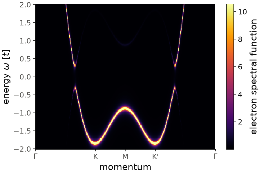
The self-consistent pairing is \(\Delta_0=0.30\), so the gap at the Fermi energy goes from \(-0.30\) to \(0.30\). Away from the Fermi energy the spectral function follows the normal band, with its minimum at K at \(-1.85\). The faint band above, with its minimum at \(0.9\) at M, is the hole copy: its electron weight is small, but not zero. ARPES measures this spectral function below the Fermi energy.

Code of this figure (documentation/figures/meanfield_swave.py)

import style
from pyqula import geometry
import numpy as np
g = geometry.triangular_lattice() # geometry of a triangular lattice
h = g.get_hamiltonian()  # get the Hamiltonian
h.setup_nambu_spinor() # setup the Nambu form of the Hamiltonian
h = h.get_mean_field_hamiltonian(U=-2.0,filling=
                   0.45,mf="swave",nk=40) # perform SCF
# electron spectral-function
(k,w,A) = h.get_kdos_bands(operator="electron",nk=400,
                   energies=np.linspace(-2.0,2.0,200),delta=0.03)
k, w, A = k.reshape(400,200), w.reshape(400,200), A.reshape(400,200)

def draw(ax, c):
    pm = ax.pcolormesh(k, w, A, cmap=c.cmap, vmax=0.5*A.max(), shading="auto")
    style.colorbar(pm, ax, "electron spectral function")
    ax.set_xticks([0, 1/3, 1/2, 2/3, 1], [r"$\Gamma$", "K", "M", "K'", r"$\Gamma$"])
    ax.set_xlabel("momentum")
    ax.set_ylabel(r"energy $\omega$ [$t$]")

style.save(draw, "meanfield_swave")
print("Delta", h.extract("swave"))
(kb,eb) = h.get_bands(); print("gap", 2*abs(eb).min())

See examples/readme_examples/scf_SC/main.py for a runnable script with a plot, and the notebook 04_anomalous_mf_sc.ipynb in the folder above.

Long-range interactions

So far the interaction was only onsite. Interactions between neighbors are needed to get charge density waves, bond order (Peierls) instabilities and unconventional superconductivity. We now take

\[ H = \sum_{\langle ij\rangle,s} c^\dagger_{i,s} c_{j,s} + h.c. + U\sum_{i} n_{i,\uparrow} n_{i,\downarrow} + V_1\sum_{\langle ij\rangle} n_i n_j , \qquad n_i = \sum_s n_{i,s}, \]

where \(U\) is the onsite interaction and \(V_1\) the interaction between first neighbors, with each bond counted once. The keywords of h.get_mean_field_hamiltonian() are:

• V1, V2, V3: the interaction between first, second and third neighbors.
• Vr: a function Vr(r1,r2) of the positions of two sites, the interaction of each pair, in the same convention as \(V_1\). A Vr equal to \(V_1\) for first neighbors and zero beyond is the same calculation as V1. The pair of a site with itself is included, so \(V_r(0)\) acts as an onsite \(U=V_r(0)\); a function meant only for bonds must return zero at zero distance.
• rcut: the range of Vr, 5 by default in a periodic system. Whole shells of pairs at the same distance are kept or dropped, so the interaction keeps the symmetry of the lattice. In a finite system all pairs are kept.

pyqula does the full Hartree-Fock decoupling: it keeps all the contractions, and with a Nambu basis also all the anomalous ones. The first-neighbor interaction \(V_1\) gives three new kinds of terms. The first is the charge (Hartree) term,

\[ H^{MF} \sim \langle n_{i,s} \rangle n_{j,s'} , \]

so the energy of a site depends on the charge of its neighbors. It gives charge density waves, with different charge on different sites. The second is the bond (Fock) term,

\[ H^{MF} \sim \langle c^\dagger_{i,s} c_{j,s} \rangle c^\dagger_{j,s} c_{i,s} + h.c., \]

which changes the hopping. If the change is not the same on all bonds, the state has a bond order, as in a Peierls distortion. The third kind are the anomalous terms,

\[ H^{MF} \sim \langle c^\dagger_{i,\uparrow} c^\dagger_{j,\uparrow} \rangle c_{j,\downarrow} c_{i,\downarrow} + h.c., \qquad \langle c^\dagger_{i,\downarrow} c^\dagger_{j,\downarrow} \rangle c_{j,\uparrow} c_{i,\uparrow} + h.c., \qquad \langle c^\dagger_{i,\uparrow} c^\dagger_{j,\downarrow} \rangle c_{j,\downarrow} c_{i,\uparrow} + h.c. \]

The first two pair electrons with the same spin, so they are odd (spin triplet). The third pairs opposite spins, and can be even or odd. So an attractive \(V_1\) can pair electrons on neighboring sites, with the same or with opposite spin, while the onsite \(U\) can only pair opposite spins on the same site.

In the example below an attractive \(V_1\) together with a large exchange field gives a spin-triplet superconductor, with \(\Delta_{\uparrow\uparrow}\) and \(\Delta_{\downarrow\downarrow}\) different from zero:

import numpy as np
from pyqula import geometry
g = geometry.triangular_lattice() # generate the geometry
h = g.get_hamiltonian() # create Hamiltonian of the system
h.add_exchange([0.,0.,1.]) # add exchange field
h.setup_nambu_spinor() # initialize the Nambu basis
# perform a superconducting non-collinear mean-field calculation
h = h.get_mean_field_hamiltonian(V1=-1.5,
                     filling=0.3,mf="random",nk=40)
# electron spectral-function
h.get_kdos_bands(operator="electron",nk=400,
                   energies=np.linspace(-2.0,2.0,200),delta=0.03)

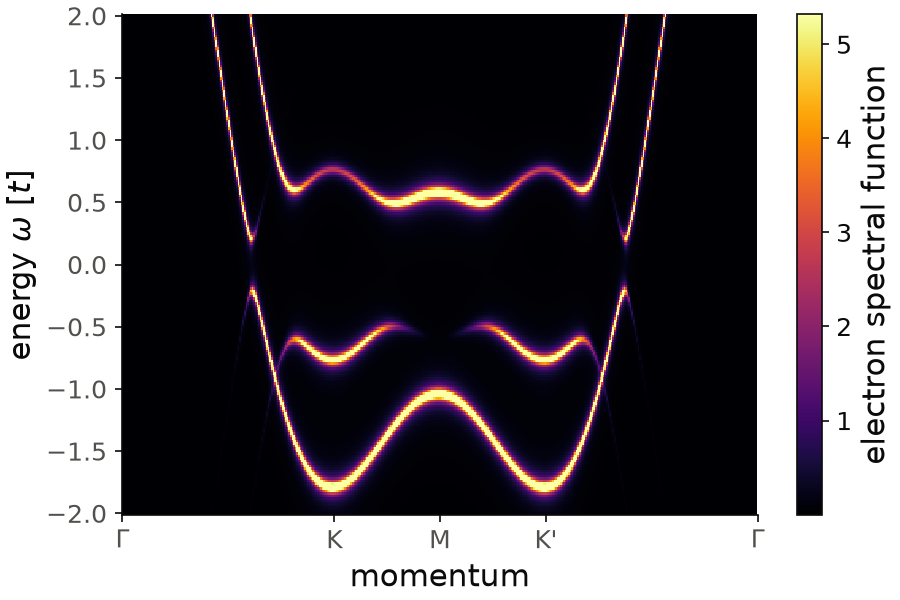
The exchange field splits the two spin bands so much that, at the Fermi energy, there are no pairs of opposite spin and opposite momentum to form a singlet. The attractive \(V_1\) then pairs electrons of the same spin on neighboring sites. The converged state has an odd, spin-triplet order parameter, and the electron spectral function shows a gap at the Fermi energy in each of the two spin-split bands. The d-vector of this state, and whether it is unitary, are computed in Superconductivity.

For the figure the loop uses nk=20 instead of nk=40, to keep it short, and the script fixes the random seed. The smallest gap is \(0.42\) with nk=20 and about \(0.40\) with nk=40, so the k-mesh changes it by a few percent. The figure shows the two copies of the triangular band, split by the exchange field. Both have a gap at the Fermi energy, and the smallest one is on the band that crosses the Fermi energy between \(\Gamma\) and K. The moment is \(-0.43\) along \(z\), opposite to the exchange vector.

Code of this figure (documentation/figures/meanfield_triplet.py)

import numpy as np
import style
from pyqula import geometry
np.random.seed(0) # fix the random guess, so that the figure is reproducible
g = geometry.triangular_lattice() # generate the geometry
h = g.get_hamiltonian() # create Hamiltonian of the system
h.add_exchange([0.,0.,1.]) # add exchange field
h.setup_nambu_spinor() # initialize the Nambu basis
# perform a superconducting non-collinear mean-field calculation
h = h.get_mean_field_hamiltonian(V1=-1.5,
                     filling=0.3,mf="random",nk=20) # nk=20 here, to keep it short
# electron spectral-function
(k,w,A) = h.get_kdos_bands(operator="electron",nk=400,
                   energies=np.linspace(-2.0,2.0,200),delta=0.03)
k, w, A = k.reshape(400,200), w.reshape(400,200), A.reshape(400,200)

def draw(ax, c):
    pm = ax.pcolormesh(k, w, A, cmap=c.cmap, vmax=0.5*A.max(), shading="auto")
    style.colorbar(pm, ax, "electron spectral function")
    ax.set_xticks([0, 1/3, 1/2, 2/3, 1], [r"$\Gamma$", "K", "M", "K'", r"$\Gamma$"])
    ax.set_xlabel("momentum")
    ax.set_ylabel(r"energy $\omega$ [$t$]")

style.save(draw, "meanfield_triplet")
(kb,eb) = h.get_bands(); print("gap", 2*abs(eb).min())
print(h.get_magnetization())
for n in ["swave"]: print(n, h.extract(n))

See examples/readme_examples/scf_SC_triplet/main.py for this calculation with a plot, examples/2d/meanfield_V1V2V3/main.py for a charge density wave driven by \(V_1\), \(V_2\) and \(V_3\) in a spinless system, and the notebook 05_full_wick_noncollinear_sc.ipynb in the folder above.