Optical conductivity

A response function tells how a system reacts to a weak perturbation. A field couples to an operator \(B\), we measure the change of an operator \(A\), and the ratio, as a function of frequency \(\omega\) and momentum transfer \(q\), is the response function \(\chi_{AB}(q,\omega)\). Its imaginary part is what a spectroscopy measures. The response pages go in three steps: the bare response of a single-particle Hamiltonian (this page and Charge response and RKKY), the same response dressed with interactions in the random phase approximation (RPA), whose poles are magnons and plasmons (Spin response and magnons), and the Bethe-Salpeter equation for excitons (Excitons).

The Kubo formula

We start with the response to an electric field, the optical conductivity tensor \(\sigma_{ab}(\omega)\) of a periodic Hamiltonian, computed with h.get_optical_conductivity(). It is given by the Kubo-Greenwood formula,

\[ \sigma_{ab}(\omega) = \frac{i e^2 \hbar}{N_k V_{\rm cell}} \sum_{\mathbf k} \sum_{n, m} \frac{f_n - f_m}{E_m - E_n} \frac{v^a_{nm} v^b_{mn}}{\hbar\omega + i\eta - (E_m-E_n)} , \]

where \(n,m\) are the bands at momentum \(\mathbf k\), \(E_n\) their energies, \(f_n\) their occupations at temperature \(T\), \(v^a_{nm}\) the matrix element of the velocity along direction \(a\), \(N_k\) the number of k-points, \(V_{\rm cell}\) the volume (area, length) of the unit cell, and \(\eta\) a broadening. The physical meaning is simple: light of frequency \(\omega\) is absorbed when it can move an electron from an occupied band to an empty band at energy \(\hbar\omega\) above, and the weight of this transition is given by the velocity matrix element.

The terms with \(E_n=E_m\) give the intraband (Drude) response. For them the factor \((f_n-f_m)/(E_m-E_n)\) is replaced by its limit \(-\partial f/\partial E\), and the result is a peak at \(\omega=0\),

\[ \sigma^{\rm intra}_{ab}(\omega) = \frac{i D_{ab}}{\omega + i\eta}, \qquad D_{ab} = \frac{1}{N_k V_{\rm cell}} \sum_{\mathbf k,n} \left(-\frac{\partial f}{\partial E}\right)_{E_n} v^a_{nn} v^b_{nn} , \]

with \(D_{ab}\) the Drude weight, available as h.get_drude_weight(). The velocity is the current operator of the tight-binding model, \(v_a = i[H, r_a]\), built from the full vector of each bond, also the bonds inside the unit cell. Because of this the tensor has the symmetry of the lattice: on the honeycomb lattice \(\sigma_{xx}=\sigma_{yy}\) exactly, and graphene gives its universal absorption \(\pi e^2/4h\) per spin.

The full complex tensor is returned. \(\mathrm{Re}\,\sigma_{xx}\) is the optical absorption. \(\sigma_{xy}\) is the magneto-optical (Kerr and Faraday) response. Its \(\omega\to0\) limit is the anomalous Hall conductivity, which for a Chern insulator with Chern number \(C\) is quantized to

\[\sigma_{xy}(0) = -C\,\frac{e^2}{h},\]

with \(C\) as returned by h.get_chern().

Units: \(\hbar=e=1\), energies in units of the hopping \(t\), lengths in units of the lattice constant. The conductivity is returned in units of \(e^2/\hbar\) (times \(a^{2-d}\) in \(d\) dimensions), so one conductance quantum \(e^2/h = e^2/(2\pi\hbar)\) is the value \(1/(2\pi)\). The Fermi energy is at zero, as everywhere in pyqula.

The absolute normalization is fixed by the f-sum rule,

\[\int_{-\infty}^{\infty} \mathrm{Re}\,\sigma_{aa}(\omega)\,d\omega = \pi W_{aa},\]

where \(W_{ab}\) is the diamagnetic weight, the occupied average of \(\partial^2 H/\partial k_a\partial k_b\), available as h.get_sum_rule_weight(). The weight is shared between the Drude peak and the interband absorption.

A Chern insulator

We take the honeycomb lattice with a Haldane term, a Chern insulator, and compute its absorption and its Hall response:

import numpy as np
from pyqula import geometry
g = geometry.honeycomb_lattice() # create a honeycomb lattice
h = g.get_hamiltonian(has_spin=False) # get the Hamiltonian
h.add_haldane(0.2) # Chern insulator
h.shift_fermi(0.3) # put the Fermi energy in the gap

(ws,s) = h.get_optical_conductivity(energies=np.linspace(0.,4.,401),
                                    nk=200,T=0.02,delta=0.05)
absorption = s[:,0,0].real # Re sigma_xx, the optical absorption

# the DC Hall response is quantized to the Chern number
(w0,s0) = h.get_optical_conductivity(energies=[0.],nk=40,T=0.01,delta=1e-3)
print("sigma_xy(0) in e^2/h:",2.*np.pi*s0[0,0,1].real) # -1

ws contains the frequencies and s the \(3\times3\) tensor at each frequency, so s has shape (len(ws),3,3). The absorption is zero below the gap and starts at the gap. The second call computes the tensor at zero frequency with a small broadening, and \(2\pi\sigma_{xy}\) comes out as \(-1\), one conductance quantum with the sign of \(-C\).

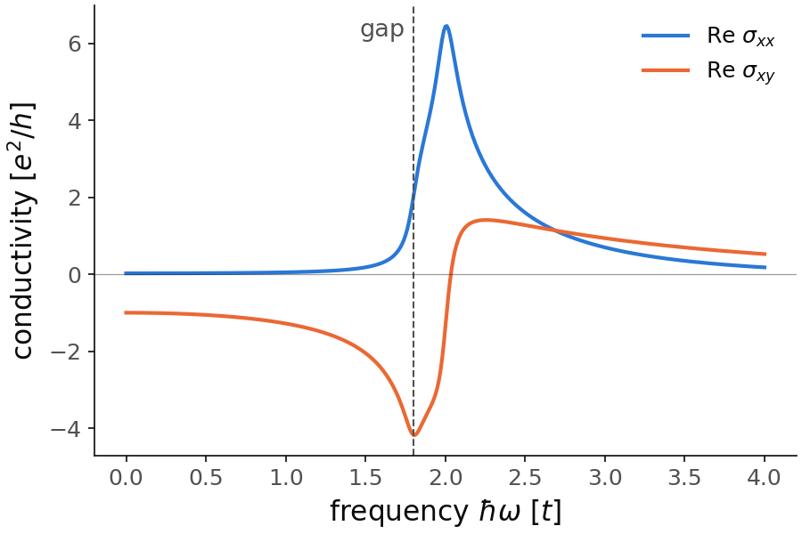
The dashed line is the band gap, \(1.8t\), from h.get_gap(). Below the gap the absorption \(\mathrm{Re}\,\sigma_{xx}\) is almost zero; the small tail comes from the broadening delta=0.05. It rises at the gap and has its maximum, \(6.45\,e^2/h\), at \(\omega=2.0t\). The Hall part \(\mathrm{Re}\,\sigma_{xy}\) starts at \(-1.00\,e^2/h\) at \(\omega=0\), the quantized value, goes down to \(-4.18\,e^2/h\) at the gap, and changes sign at \(\omega=2.03t\), next to the maximum of the absorption. With delta=0.05 the k-mesh has to be fine: at nk=40 both curves have wiggles above the gap, which are the separate k-points of the mesh. At nk=200 they are gone, and nk=300 changes the curves by less than \(2\times10^{-4}\,e^2/h\).

Code of this figure (documentation/figures/optical_chern.py)

import numpy as np
import style
from pyqula import geometry
g = geometry.honeycomb_lattice() # create a honeycomb lattice
h = g.get_hamiltonian(has_spin=False) # get the Hamiltonian
h.add_haldane(0.2) # Chern insulator
h.shift_fermi(0.3) # put the Fermi energy in the gap

(ws,s) = h.get_optical_conductivity(energies=np.linspace(0.,4.,401),
                                    nk=200,T=0.02,delta=0.05)
absorption = s[:,0,0].real # Re sigma_xx, the optical absorption

# the DC Hall response is quantized to the Chern number
(w0,s0) = h.get_optical_conductivity(energies=[0.],nk=40,T=0.01,delta=1e-3)
print("sigma_xy(0) in e^2/h:",2.*np.pi*s0[0,0,1].real) # -1

gap = h.get_gap() # the band gap, to mark the absorption edge

def draw(ax, c):
    ax.plot(ws, 2*np.pi*absorption, color=c.blue,
            label=r"Re $\sigma_{xx}$")
    ax.plot(ws, 2*np.pi*s[:,0,1].real, color=c.orange,
            label=r"Re $\sigma_{xy}$")
    ax.axvline(gap, color=c.ink2, lw=1.0, ls="--")
    ax.text(gap-0.05, 0.97, "gap", color=c.ink2, va="top", ha="right",
            transform=ax.get_xaxis_transform())
    ax.axhline(0, color=c.ink, lw=0.6, alpha=0.4)
    ax.set_xlabel(r"frequency $\hbar\omega$ [$t$]")
    ax.set_ylabel(r"conductivity [$e^2/h$]")
    ax.legend(loc="upper right")

style.save(draw, "optical_chern")

The keywords are

• energies: the frequencies \(\hbar\omega\).
• nk: number of k-points per direction. A small delta needs a large nk, otherwise the absorption shows the discrete k-mesh.
• T: temperature of the Fermi function.
• delta: the broadening \(\eta\).
• intraband, interband: switch on or off the Drude part and the interband part.

The formula works for one- and two-dimensional Hamiltonians. Superconducting (Nambu) Hamiltonians and three-dimensional ones raise NotImplementedError; for a Nambu Hamiltonian the hole block carries the opposite charge, so the current is not \(i[H,r]\).

See examples/2d/optical_conductivity/main.py and examples/1d/optical_conductivity_chain/main.py for runnable scripts, and 01_optical_conductivity.ipynb and 02_drude_weight_f_sum_rule.ipynb in jupyter-notebooks/functionalities/response_functions/ for executed notebooks.