Local density of states

In this page we resolve the density of states in space. This is the quantity that STM measures: the differential conductance \(dI/dV\) at bias \(V\) and tip position \(\mathbf r\) is, in a first approximation, proportional to the local density of states at energy \(eV\) and position \(\mathbf r\).

Local density of states at one energy

The local density of states on site \(n\) is

\[ D(\omega,n) = \frac{1}{N_k}\sum_{k,\alpha} \delta(\omega-\epsilon_{k,\alpha})\, | \langle n | \Psi_{k,\alpha} \rangle |^2 , \]

where \(\epsilon_{k,\alpha}\) are the eigenenergies, \(\langle n | \Psi_{k,\alpha}\rangle\) is the amplitude of the eigenstate on site \(n\), and the delta function is broadened with a Lorentzian of width \(\delta\). It counts the states at energy \(\omega\), each one weighted by its probability on site \(n\). The sum over all the sites gives back the density of states of Band structures and DOS. We compute it with h.get_ldos():

from pyqula import geometry
g = geometry.honeycomb_zigzag_ribbon() # get the geometry
h = g.get_hamiltonian()  # get the Hamiltonian
(x,y,d) = h.get_ldos()

h.get_ldos() returns three arrays: the \(x\) and \(y\) coordinates of the sites, and the local density of states on each site, at the energy e (zero by default). For a periodic system the unit cell is repeated a few times, so the map is easier to see. For the zigzag ribbon at zero energy, about three quarters of the weight is on the outermost sites of the two edges. These are the zigzag edge states, and this profile is what STM measures at a zigzag edge of graphene.

The keywords are

• e: the energy \(\omega\).
• delta: the broadening \(\delta\).
• operator: weight each state with an operator, for example "sz" for a map of the spin density of states instead of the charge one.
• mode: "arpack" (default, diagonalization on a k-mesh), "green" (Green's function, 2D only) or "KPM" (Chebyshev expansion, for large systems, see Kernel polynomial method).
• projection: "TB" (default, one value per site), "TBRS" (the same values, interpolated on a continuous grid in real space) or "atomic" (each site replaced by an atomic orbital, which gives a smooth map closer to an STM image).
• num_bands: compute only this many states around e, for large Hamiltonians.

With an operator \(A\), the two modes do not compute exactly the same thing. mode="arpack" weights each eigenstate with its expectation value, \(\langle\Psi|A|\Psi\rangle\,|\Psi(n)|^2\). mode="green" and mode="KPM" use the local matrix element \(\textrm{Re}\,\Psi^*(n)(A\Psi)(n)\). The two agree for a state that is an eigenstate of \(A\), and summed over the sites both give the same total. For a state whose spin, say, changes from site to site, only the local matrix element shows this change in the map. An operator that depends on momentum, such as "valley", only works with mode="arpack", because the Green's function has already summed over the Brillouin zone.

For a smoother map than one value per site, use projection="TBRS":

from pyqula import geometry
g = geometry.honeycomb_zigzag_ribbon() # get the geometry
h = g.get_hamiltonian()  # get the Hamiltonian
(x,y,d) = h.get_ldos(e=0.0,projection="TBRS") # interpolated real-space map

To follow how the map changes with energy, as in a series of STM conductance maps at different biases, h.get_multildos() computes the local density of states at many energies at once:

import numpy as np
(x,y,es,ldos) = h.get_multildos(energies=np.linspace(-2.0,2.0,100),projection="atomic") # one map per energy

x and y are the positions, es the energies, and ldos has one row for each energy, so the rows are the frames of a stack \(D(x,y,\omega)\). The maps are also written to the folder MULTILDOS/, one file per energy, together with the total density of states in MULTILDOS/DOS.OUT, unless write=False is given. DOS.OUT has the same normalization as h.get_dos(). With the default projection, projection="TB", the maps have the same normalization as h.get_ldos(), and the sum of a map over the sites is the density of states at that energy. With projection="atomic" the map is a density on a continuous grid in real space. Each eigenstate is written in real space as \(\Psi(\mathbf r)=\sum_n \Psi(n)\,\phi(\mathbf r-\mathbf r_n)\), with \(\phi(\mathbf r)=e^{-|\mathbf r|/1.5}\) an atomic orbital, and the map is \(|\Psi(\mathbf r)|^2\). The orbitals of neighboring sites overlap, so \(|\Psi(\mathbf r)|^2\) also contains the interference between them. For this reason each state is normalized on the grid, before the broadening: the integral of its map, the sum over the grid times the area of one grid cell, is the weight the state has in the map of projection="TB". The shape of each state does not change. As a result, the integral of an atomic map is the density of states at that energy, as the sum of a map with projection="TB", and the intensities at different energies can be compared. For the zigzag ribbon with delta=0.1 and nk=200, the integral of the atomic map is 13.3 at both \(\omega=-2t\) and \(\omega=2t\), the same as the sum of the tight-binding map, because the density of states is the same at the two energies. The interference is still in the shape: the maximum of the map is 2.6 times higher at \(\omega=-2t\) than at \(\omega=2t\). With an operator, h.get_multildos() uses the expectation value \(\langle\Psi|A|\Psi\rangle\) times \(|\Psi(n)|^2\), as mode="arpack" above. projection="atomic" does not accept an operator.

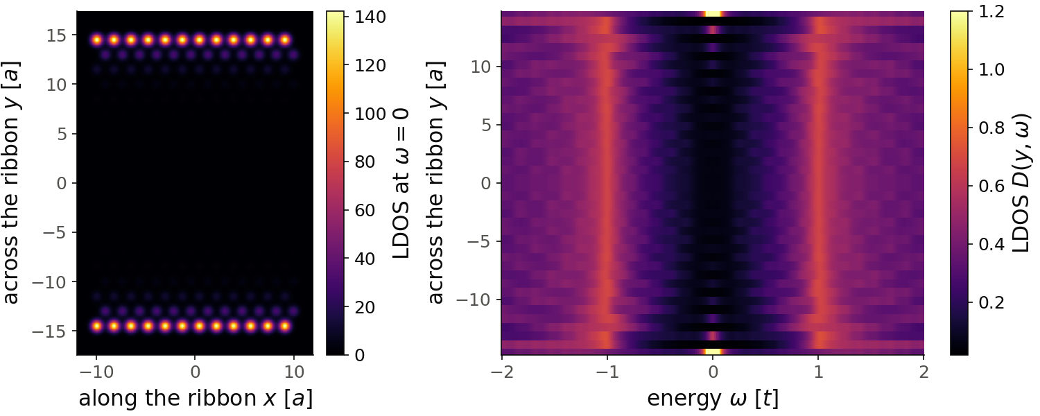
In both panels the position across the ribbon is the vertical axis. On the left, the map at zero energy with projection="TBRS", with the ribbon along the horizontal axis. We take nrep=12, twelve unit cells of the ribbon, so that the map is not a thin strip. Lengths are in units of the first-neighbor distance \(a\). The weight is on the outermost sites of the two edges, and it decays into the ribbon on every second site, on one sublattice only. On the right, the maps of h.get_multildos() at 401 energies, one column per energy, as a stack of STM maps. Here we use the default projection, one value per site, instead of projection="atomic", so that each row is one site. We take nk=1000 and delta=0.05. With the default nk=100 and delta=0.01 the map is speckled, for two reasons. The first is the k-mesh: the broadening is smaller than the energy step between neighboring k-points. At nk=1000 this is gone, and nk=3000 changes the map by less than \(10^{-5}\). The second is physical: the ribbon has 40 sites in its unit cell, so 40 subbands, and the edge of each subband gives a sharp peak in energy. The larger delta=0.05 smooths them, as the finite energy resolution of an STM does. You see a bright line at \(\omega=0\) on the edge sites, with the value \(2.8\), against \(0.60\) on the next site of the same sublattice and almost zero on the other sublattice. Away from zero energy the weight spreads over the whole ribbon, with the bulk van Hove peaks at \(\pm t\). The alternation from one row to the next is the sublattice.

Code of this figure (documentation/figures/ldos_zigzag.py)

import numpy as np
import style
from pyqula import geometry

g = geometry.honeycomb_zigzag_ribbon() # get the geometry
h = g.get_hamiltonian()  # get the Hamiltonian
(x,y,d) = h.get_ldos(e=0.0,projection="TBRS",nrep=12) # interpolated real-space map, 12 unit cells long
(x2,y2,es,ldos) = h.get_multildos(energies=np.linspace(-2.0,2.0,401),
                                  nk=1000,delta=0.05) # one map per energy, one value per site

d = d.reshape(600,600) # TBRS gives a 600 x 600 grid, x first
iy = np.argsort(y2) # sites ordered across the ribbon

def draw(ax, c):
    # the position across the ribbon is the vertical axis of both panels
    im = ax[0].pcolormesh(np.unique(x), np.unique(y), d.T, cmap=c.cmap, shading="auto")
    style.colorbar(im, ax[0], r"LDOS at $\omega=0$")
    ax[0].set_aspect("equal")
    ax[0].set_xlabel("along the ribbon $x$ [$a$]")
    ax[0].set_ylabel("across the ribbon $y$ [$a$]")
    im = ax[1].pcolormesh(es, y2[iy], ldos[:,iy].T, cmap=c.cmap, shading="nearest", vmax=1.2)
    style.colorbar(im, ax[1], r"LDOS $D(y,\omega)$")
    ax[1].set_xlabel(r"energy $\omega$ [$t$]")
    ax[1].set_ylabel("across the ribbon $y$ [$a$]")

style.save(draw, "ldos_zigzag", npanels=2, gridspec_kw={"width_ratios":[1,1.6]})

See examples/0d/island/main.py for a runnable script on a superconducting island with projection="TBRS".

Local density of states of a finite island

On a finite island the states are discrete, and the map at each energy shows one or a few of them. For a triangular island of the honeycomb lattice, we compute the maps at many energies with h.get_multildos():

from pyqula import islands
g = islands.get_geometry(name="honeycomb",n=3,nedges=3) # get an island
h = g.get_hamiltonian() # get the Hamiltonian
h.get_multildos(projection="atomic") # get the LDOS

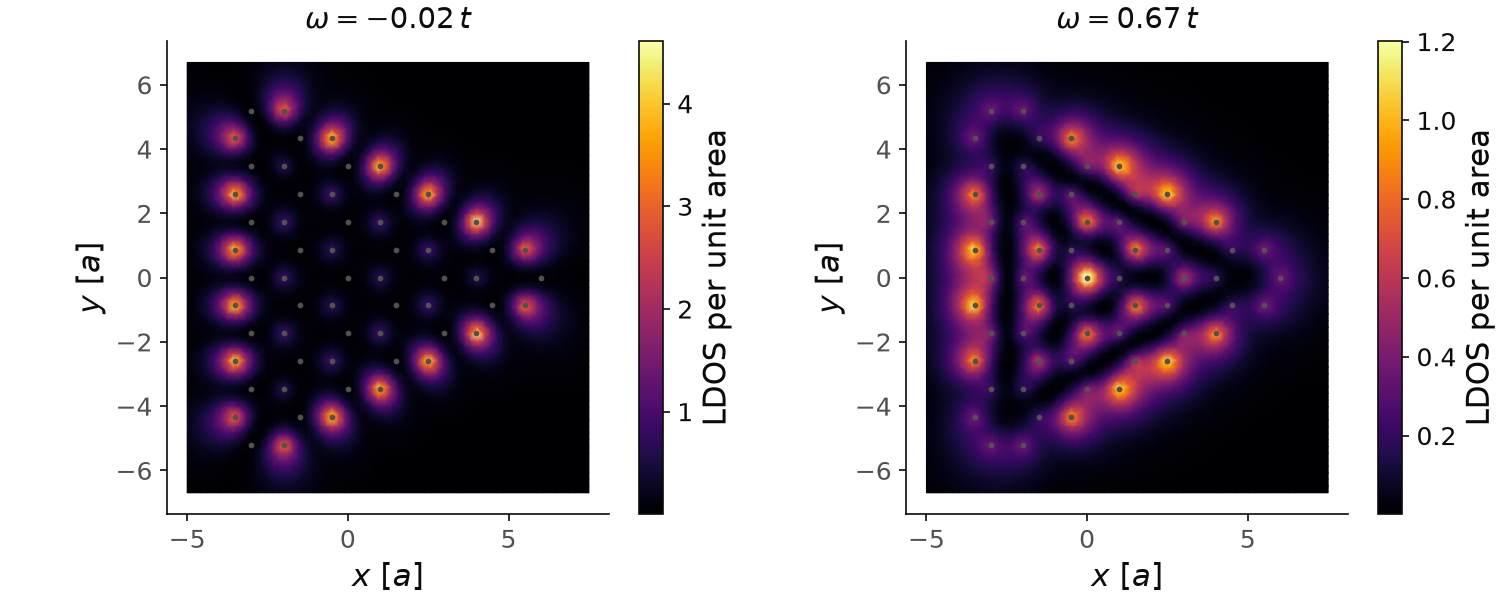
The island has 61 sites. Its Hamiltonian has five zero-energy states, the difference between the number of sites of the two sublattices. On the left, the map at \(\omega=-0.02t\), the energy of the grid closest to zero, shows these states: the weight is on the outer sites of the three zigzag edges, on one sublattice, and it is almost zero inside. On the right, at the first level above them, \(\omega=0.67t\), the weight is spread over the inside of the island, with a node line between the edge and the center. The small dots are the sites. Here we assign the output of h.get_multildos() to arrays, which the snippet above does not do.

Code of this figure (documentation/figures/ldos_island.py)

import numpy as np
import style
from pyqula import islands

g = islands.get_geometry(name="honeycomb",n=3,nedges=3) # get an island
h = g.get_hamiltonian() # get the Hamiltonian
(x,y,es,ldos) = h.get_multildos(projection="atomic") # get the LDOS

def draw(ax, c):
    for a, e0 in zip(ax, [0.0, 0.67]): # zero modes, and the first level above
        i = np.argmin(np.abs(es-e0)) # the frame closest to e0
        im = a.tripcolor(x, y, ldos[i], cmap=c.cmap, shading="gouraud")
        style.colorbar(im, a, "LDOS per unit area")
        a.scatter(g.x, g.y, s=3, color=c.ink2)
        a.set_aspect("equal")
        a.set_title(r"$\omega=%.2f\,t$" % es[i])
        a.set_xlabel("$x$ [$a$]")
        a.set_ylabel("$y$ [$a$]")

style.save(draw, "ldos_island", npanels=2)

The map at each energy is what STM measures on the island at that bias, and DOS.OUT is the spectrum of the whole island. See examples/readme_examples/ldos_island/main.py for a runnable script that plots the maps.