Long-range modulations: the ultracell

In this page we compute a crystal whose density or magnetization changes slowly over many unit cells, for example a spin density wave, a screened impurity or a domain wall. We first apply a potential over eight cells of silicon and see the electrons screen it. Then we compute the energy of the modulation, a spin density wave, and what a scanning-tunnelling microscope sees above it. We end with what tunnels through a modulated sheet and with a magnetic texture that the calculation keeps without any field.

A modulation over many cells

A spin density wave in chromium repeats every 21 unit cells, and a skyrmion is hundreds of cells across. In both cases the crystal is still periodic on the scale of the atoms, and only a slow envelope changes from cell to cell. A supercell pays for the envelope the same price as for the atoms, so we do something else. We take \(N = n_1 n_2 n_3\) copies of the unit cell, the long cell or ultracell. Its reciprocal lattice vectors inside the Brillouin zone of the unit cell are \(N\) wavevectors \(\mathbf Q\), and the density is written as

\[ \rho(\mathbf r) = \sum_{\mathbf Q} \rho_{\mathbf Q}(\mathbf r)\, e^{i\mathbf Q\cdot\mathbf r}, \]

with each \(\rho_{\mathbf Q}\) periodic on the unit cell. A state of the long cell is expanded in the Kohn-Sham states of the unit cell at the \(N\) k-points that fold onto the same point of the long cell:

\[ |\Psi_{\mathbf k}\rangle = \sum_{\mathbf Q}\sum_{n=1}^{n_{\rm bnd}} c_{\mathbf Q n}\,|\psi_{\mathbf k + \mathbf Q, n}\rangle . \]

The unit-cell states are computed once, and the self-consistent loop then diagonalizes a small dense matrix of size \(N n_{\rm bnd}\) at each k-point of the long cell. When nbnd grows, this basis becomes the full plane-wave basis of the supercell, so the method is a variational truncation of the real supercell, and nbnd is its one convergence parameter. For an insulator the default nbnd has no empty bands, which leaves the envelope nothing to be built from, so you always give it. Each number on this page is at one value of nbnd and on a small k-mesh of the long cell, for example nbnd=32 on a \(1\times2\times2\) mesh of the long cell for silicon at ecutwfc = 12, and none of them is converged. You check them by raising nbnd and kgrid.

Here we take silicon and apply a potential \(V(\mathbf r) = 0.02\cos(2\pi x_1/8)\) Ry, one period over eight cells along \(\mathbf a_1\). We compute it with calc.get_ultracell():

import numpy as np
from defuqumat import Calculator

calc = Calculator.from_file("docs/figures/ultracell_sdw/si.in",
                            pseudo_dir="tests/data/pseudo")
applied = lambda x: 0.02 * np.cos(2 * np.pi * x[..., 0] / 8)   # Ry, x in unit cells
ulr = calc.get_ultracell(supercell=(8, 1, 1), kgrid=(1, 2, 2), nbnd=32,
                         external=applied)
print(f"{ulr.iterations} iterations, converged {ulr.converged}")
print(ulr.density.shape)                     # (spin, grid of the long cell)
print(f"largest induced density {np.abs(ulr.modulation).max():.3e} e/bohr^3")

dv = np.asarray(ulr.delta_v[0]).mean(axis=(1, 2))     # plane average along a1
felt = 2 * np.abs(np.fft.rfft(dv)[1]) / dv.size        # its cosine component
print(f"applied 20.00 mRy, felt {1000 * felt:.2f} mRy")

9 iterations, converged True
(1, 120, 15, 15)
largest induced density 7.647e-05 e/bohr^3
applied 20.00 mRy, felt 2.00 mRy

supercell is the number of unit cells along each lattice vector, and kgrid is the k-mesh of the long cell. The k-mesh of the input must be supercell times kgrid, here \(8\times2\times2\), because the long cell folds onto exactly these points. external is the applied potential in Ry, as a function of the crystal coordinates of the unit cell, which run from 0 to \(n_i\) across the long cell. ulr.density is the density on the grid of the whole long cell, and ulr.modulation is its difference from the uniform crystal. ulr.delta_v is the change of the potential that an electron feels, the applied potential plus the Hartree and exchange-correlation potential of the induced charge.

The loop converges in 9 iterations, and the density is on a grid of \(120\times15\times15\) points, which is eight times the grid of the unit cell along \(\mathbf a_1\). The largest change of the density is \(7.6\times10^{-5}\) e/bohr\(^3\), so the modulation is small, as it should be for a potential of 20 mRy. What the electrons feel is the cosine component of the plane average of delta_v, and it is 2.00 mRy, ten times smaller than what we apply. This is screening: the induced charge builds a Hartree potential that almost cancels the applied one. The ratio of the two, here 10, is roughly the static dielectric function of silicon at the wavevector of one period over eight cells. It is only roughly this, because delta_v also holds the exchange-correlation potential of the induced charge. The value 10 is also below the converged LDA value, because nbnd=32 and the \(1\times2\times2\) mesh of the long cell are not converged.

The energy of a modulation

We now ask whether a modulation costs or gains energy. ulr.total_energy is the Kohn-Sham energy per unit cell of the long cell, and the uniform crystal, the normal SCF, is its reference:

uniform = calc.get_scf().total_energy
print(f"uniform   {uniform:.8f} Ry per cell")
print(f"modulated {ulr.total_energy:.8f} Ry per cell")
print(f"change {1000 * (ulr.total_energy - uniform):+.5f} mRy per cell")

uniform   -15.71359794 Ry per cell
modulated -15.71361495 Ry per cell
change -0.01701 mRy per cell

The modulated crystal is 0.017 mRy per cell below the uniform one. This does not mean that the uniform crystal is unstable. The applied potential external is part of the Hamiltonian, so its energy \(\int V\rho\) is inside total_energy, and the electrons always lower this energy when they move towards the low potential. This is the screening energy, which is second order in \(V\) and always negative. The test for a state with no applied potential, where the sign does say which state is the ground state, is in the section "A texture that the calculation keeps".

Since the bases are nested in nbnd, the energy approaches the energy of the real supercell from above as nbnd grows. This makes it the quantity that says whether a modulated state is the ground state: a spin density wave or a charge density wave is stable only if its energy is below that of the uniform state. Under a magnetic field the energy of the field is not in total_energy, as in the rest of the code, and it is in ulr.field_energy. So when you compare two states under a field, you compare total_energy + field_energy.

A spin density wave

We now apply a magnetic field that changes sign over the long cell. With nspin = 2 the field enters as \(v_\uparrow - B\) and \(v_\downarrow + B\), and the two spin channels share one Fermi level, so spin-up electrons can gather in the cells where the field favours them and spin-down electrons in the others. This is what a spin density wave is made of. The silicon cell has no moment of its own, so the moment we get is the spin response of the crystal at the wavevector of the field, the \(\mathbf Q\)-resolved spin susceptibility:

magnet = Calculator.from_file("docs/figures/ultracell_sdw/si-mag.in",
                              pseudo_dir="tests/data/pseudo")
field = lambda x: 0.02 * np.cos(2 * np.pi * x[..., 0] / 8)     # Ry
wave = magnet.get_ultracell(supercell=(8, 1, 1), kgrid=(1, 2, 2), nbnd=32,
                            magnetic_field=field)
print(f"{wave.iterations} iterations, converged {wave.converged}")
print(np.round(wave.cell_moments(), 4))       # mu_B, one value per unit cell
print(f"field energy {1000 * wave.field_energy:.4f} mRy per cell")

8 iterations, converged True
[ 0.1194  0.0471 -0.0473 -0.1223 -0.1194 -0.0471  0.0473  0.1223]
field energy -1.2949 mRy per cell

The loop converges in 8 iterations. wave.cell_moments() is the moment of each of the eight unit cells, and it follows the field, from \(+0.122\) \(\mu_B\) where the field is largest to \(-0.122\) \(\mu_B\) four cells later, with \(\pm0.047\) \(\mu_B\) in between. The total moment is zero, so this is a spin density wave and not a ferromagnet. The moment comes from the same mixing of valence and conduction states that screens the potential in the first section, now with opposite signs in the two spin channels. The gaussian smearing of 0.02 Ry in the input only adds a small part from the tails of the band edges. field_energy is \(-\int\mathbf B\cdot\mathbf m\), \(-1.29\) mRy per cell here, and you add it to total_energy when you compare this state with another one under the same field.

What a tip sees

What does a scanning-tunnelling microscope see above a spin density wave? In the Tersoff-Hamann picture the current is the local density of states at the tip, at the energy that the bias selects:

\[ I(\mathbf r_{\rm tip}) \propto \sum_{n\mathbf k} |\Psi_{n\mathbf k}(\mathbf r_{\rm tip})|^2\, \delta_w(\varepsilon_{n\mathbf k} - E_F - eV) , \]

with \(\delta_w\) a delta function smeared by the width \(w\). A tip with a moment sees only one spin channel, and a normal tip sees the sum of the two. We compute the image with calc.get_ultracell_stm(), on the same magnet as above:

plane = dict(height=0.35, axis=2, shape=(96, 12))
charge = magnet.get_ultracell_stm(**plane)
up = magnet.get_ultracell_stm(spin="up", **plane)

def per_cell(image):           # the image averaged over each unit cell
    c = np.asarray(image.values).mean(axis=1).reshape(8, -1).mean(axis=1)
    return c / c.mean()

print("unpolarized tip", np.round(per_cell(charge), 3))
print("tip up         ", np.round(per_cell(up), 3))

unpolarized tip [1.167 0.817 0.829 1.188 1.167 0.817 0.829 1.188]
tip up          [1.496 0.946 0.717 0.872 0.838 0.687 0.941 1.503]

The image is a plane at the crystal coordinate height along axis, in the units of the unit cell, and it spans the whole long cell, here with 96 points along the eight cells. Bulk silicon has no surface, so this plane cuts through the crystal, and the image is the local density of states inside it. With no bias the tip energy is the Fermi level, which is in the gap of silicon, so the image comes from the tails of the band edges. spin="up" gives a fully polarized tip, and polarization sets a smaller polarization. For a polarized tip the current changes by 82 per cent of its mean from cell to cell, from 1.503 to 0.687, with one period over the eight cells. For an unpolarized tip it changes by 37 per cent, from 1.188 to 0.817, with two periods. The reason is symmetry: if we flip every spin and the sign of the field together, the crystal does not change, so the charge cannot depend on the sign of the field and it only sees the square of the wave, which has twice its wavevector.

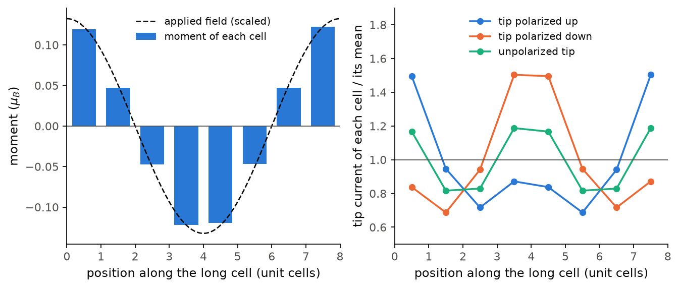
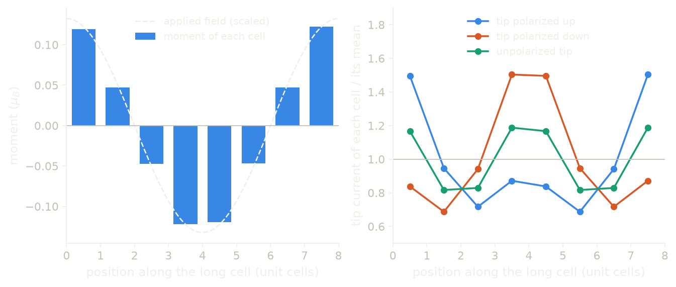
The left panel shows the moment of each cell and the applied field, scaled to the same height, and we see that the moment follows the field with the same sign, from \(+0.122\) to \(-0.122\) \(\mu_B\). The right panel shows the tip current of each cell for the three tips. The tip polarized up is brightest in cells 1 and 8, where the moment is up, and the tip polarized down gives the same curve moved by four cells, half a period. The unpolarized tip is brightest where the moment is largest in size, in cells 1, 4, 5 and 8, so its period is four cells. The polarized curve is not a pure cosine, because it is the spin part with one period plus this charge part with two, and so its minima, 0.687 and 0.717, are in cells 6 and 3 rather than in cells 4 and 5.

Code of this figure (docs/figures/ultracell_sdw/)

compute.py

"""A spin density wave over eight cells of silicon, and what a tip sees above it."""
import numpy as np
from defuqumat import Calculator
from common import PSEUDO, save

calc = Calculator.from_file("si-mag.in", pseudo_dir=PSEUDO)
field = lambda x: 0.02 * np.cos(2 * np.pi * x[..., 0] / 8)    # Ry, x in unit cells
wave = calc.get_ultracell(supercell=(8, 1, 1), kgrid=(1, 2, 2), nbnd=32,
                          magnetic_field=field)

# STM images on a plane across the eight cells, for three tips
plane = dict(height=0.35, axis=2, shape=(96, 12))
images = {name: np.asarray(calc.get_ultracell_stm(spin=spin, **plane).values)
          for name, spin in (("charge", None), ("up", "up"), ("down", "down"))}

cells = np.arange(8) + 0.5
m = np.asarray(wave.magnetization)
save(cells=cells, moments=wave.cell_moments(), field=field(cells[:, None]),
     x=np.arange(m.shape[0]) * 8 / m.shape[0], profile=m.mean(axis=(1, 2)),
     iterations=wave.iterations, **images)

plot.py

"""The spin density wave of silicon, and the tip current above it."""
import numpy as np
import style

d = np.load("data.npz")


def draw():
    fig, (a, b) = style.figure(2)
    scale = np.abs(d["moments"]).max() / np.abs(d["field"]).max()
    a.bar(d["cells"], d["moments"], width=0.7, color=style.color(0),
          label="moment of each cell")
    x = np.linspace(0, 8, 200)
    a.plot(x, scale * 0.02 * np.cos(2 * np.pi * x / 8), **style.reference(),
           label="applied field (scaled)")
    style.zero_line(a)
    a.set_xlim(0, 8)
    a.set_xlabel("position along the long cell (unit cells)")
    a.set_ylabel(r"moment ($\mu_B$)")
    a.legend(loc="upper center")

    for k, (name, label) in enumerate((("up", "tip polarized up"),
                                       ("down", "tip polarized down"),
                                       ("charge", "unpolarized tip"))):
        cell = d[name].mean(axis=1).reshape(8, -1).mean(axis=1)
        b.plot(d["cells"], cell / cell.mean(), "o-", color=style.color(k),
               label=label)
    b.axhline(1.0, color=style.ink2(), lw=0.8)
    b.set_xlim(0, 8)
    b.set_ylim(0.5, 1.9)
    b.set_xlabel("position along the long cell (unit cells)")
    b.set_ylabel("tip current of each cell / its mean")
    b.legend(loc="upper center", ncol=1)
    return fig


style.main(draw)

An image is one energy, and a spectrum at each point shows where in energy the states move. We compute \(dI/dV\) with calc.get_ultracell_sts(), here at the centre of each cell and for 41 energies within 0.06 Ry of the Fermi level:

RY = 13.605693                  # eV
tips = np.stack([np.arange(8) + 0.5, np.full(8, 0.5), np.full(8, 0.35)], axis=-1)
bias = wave.fermi_energy + np.linspace(-0.06, 0.06, 41)
for spin in ("up", "down"):
    sts = magnet.get_ultracell_sts(energies=bias, tip=tips, width=0.02, spin=spin)
    peak = sts.bias_axis[np.argmax(np.asarray(sts.values), axis=0)]
    print(spin, sts.values.shape, np.round(peak * RY, 2))

up (41, 8) [0.29 0.37 0.49 0.57 0.53 0.49 0.41 0.24]
down (41, 8) [0.53 0.49 0.41 0.24 0.29 0.37 0.49 0.57]

energies are the tip energies in Ry, tip gives the tip positions in the crystal coordinates of the unit cell, and sts.values has one row per energy and one column per tip. sts.bias_axis is the energy measured from the Fermi level, which is the bias of the experiment. In this window the largest \(dI/dV\) comes from the conduction states just above the gap, and we see that it moves through the wave. For spin up it is at 0.24 eV in cell 8, where the moment is largest, and at 0.57 eV in cell 4, so it moves by 0.33 eV. The peak is read on an energy axis with a step of 0.003 Ry, which is 0.04 eV, so this shift is known to about that step. For spin down it is the same curve moved by four cells. This shift in energy is the local exchange splitting that a spin-polarized STS measurement fits, and an image at one bias cannot give it, because a level that moves and a level that gains weight look the same at one energy.

Tunnelling through the modulation

An image says what the tip sees. We now ask what goes through a sheet, which is what a vertical tunnelling junction measures: the electron enters at a point \(\mathbf r\) above the sheet and leaves into an infinite, featureless substrate, a plane below it. The current is then given by the Green's function between the tip and the plane, not by the density of states at one point:

\[ T(\mathbf r; E) \propto \int_{\rm plane} d^2 r'\, \big|G(\mathbf r, \mathbf r'; E)\big|^2 . \]

The two maps differ where several states have the same energy, because these states interfere on their way through the sheet. Here we take a square sheet of silicon atoms in vacuum, with a PAW dataset, and apply a potential with one period over two cells, \(V = 0.05\cos(\pi x_1)\) Ry, so that the two atoms of the long cell are different. We compute the transmission with calc.get_ultracell_transport():

sheet = Calculator.from_file("docs/figures/ultracell_sdw/si-sheet-paw.in",
                             pseudo_dir="tests/data/pseudo")
sheet.get_ultracell(supercell=(2, 1, 1), kgrid=(2, 4, 1), nbnd=12,
                    external=lambda x: 0.05 * np.cos(np.pi * x[..., 0]))
t = sheet.get_ultracell_transport(exit_height=0.15, height=0.85, axis=2,
                                  shape=(12, 4), broadening=0.05)
image = sheet.get_ultracell_stm(height=0.85, axis=2, shape=(12, 4))
print(t.values.shape)
for name, v in (("transmission", t.values), ("image", image.values)):
    line = np.asarray(v).mean(axis=1)
    print(f"{name:12s}", np.round(line / line.mean(), 3))

(12, 4)
transmission [1.105 1.008 0.83  0.785 0.941 1.21  1.346 1.21  0.941 0.785 0.83  1.008]
image        [1.144 1.046 0.859 0.796 0.923 1.162 1.282 1.162 0.923 0.796 0.859 1.046]

The images, spectra and transmissions use the last get_ultracell() of the same calculator, so we call it first and then ask for the maps. exit_height is the crystal coordinate of the substrate plane, below the sheet at 0.5, and height is the tip plane above it, both outside the augmentation sphere of the atom. broadening is the width in Ry of the energy window at the Fermi level. Each line is the map averaged across the sheet, at 12 points along the two cells, in units of its mean. Both maps are brightest on the atoms, at the first and the seventh point, and the atom under the attractive half of the potential, at \(x_1 = 1\), is the brighter one. The transmission has the larger contrast between the two atoms, 1.346 against 1.105, where the image has 1.282 against 1.144. Part of this difference comes from the interference between the states at the Fermi level, which the image does not contain, but the two maps also differ in the propagation to the exit plane and in their energy window, and we did not separate these. The cell is small and the k-mesh of the long cell is \(2\times4\), so these numbers show what the call gives rather than a converged map of a real material.

A texture that the calculation keeps

We now compute an ordered state rather than a response. Nothing in a self-consistent calculation breaks the spin symmetry by itself, so a long cell built from a ferromagnetic unit cell stays ferromagnetic: the tiled state is an exact solution of the equations of the long cell, however long it is. To reach a wave we give the loop a starting texture with seed_magnetization. This is a factor \(s(\mathbf r)\) on the moment that the unit cell already has, with \(|s| \le 1\), the same role that starting_magnetization has for one atom:

\[ \mathbf m(\mathbf r) \;\to\; |s(\mathbf r)|\, R\big(\hat{\mathbf e}_0 \to \hat s(\mathbf r)\big)\,\mathbf m_0(\mathbf r) , \]

which is \(m \to s\,m_0\) for a collinear run. No field is applied, so the loop keeps the texture only if it is a self-consistent solution. Here we take a simple cubic lattice of hydrogen atoms, collinear, with a moment on each atom, and we seed one period over two cells, which puts the two atoms antiparallel:

import numpy as np
from defuqumat import Calculator

h = Calculator.from_file("docs/figures/ultracell_sdw/h-mag.in",
                         pseudo_dir="tests/data/pseudo")
print(f"unit cell {h.get_scf().magnetization:.4f} mu_B")
tiled = h.get_ultracell(supercell=(2, 1, 1), kgrid=(2, 2, 2), nbnd=24)
print(f"{tiled.iterations} iteration(s), cells", np.round(tiled.cell_moments(), 4))

stagger = lambda x: np.cos(np.pi * (x[..., 0] - 0.5))    # +1 and -1 at the atoms
wave = h.get_ultracell(supercell=(2, 1, 1), kgrid=(2, 2, 2), nbnd=24,
                       seed_magnetization=stagger)
print(f"{wave.iterations} iterations, cells", np.round(wave.cell_moments(), 4))
print(f"gain {1000 * (tiled.total_energy - wave.total_energy):.3f} mRy per cell")

unit cell 0.6234 mu_B
1 iteration(s), cells [0.6234 0.6234]
8 iterations, cells [ 0.4148 -0.4147]
gain 3.017 mRy per cell

cell_moments() gives the moment of each unit cell of the long cell, in \(\mu_B\), which needs no sphere because the cells fill the long cell exactly. Without a seed the loop stops after one iteration at the tiled ferromagnet, 0.6234 \(\mu_B\) in each cell, which is the moment of the unit cell. With the seed it converges in 8 iterations to the antiferromagnet, with \(\pm 0.415\) \(\mu_B\) per cell, and this state is 3.017 mRy per cell below the ferromagnet. So here the energy says which of the two solutions is lower, and the seed is only how we reach the second one. The value 3.017 mRy is at nbnd=24 on a \(4\times2\times2\) mesh, and it is not converged.

For a texture that turns we use a noncollinear cell, and the seed is then a vector at each point. Here the moment of the unit cell points along \(x\), and we seed a helix that turns by 90 degrees per cell in the \(yz\) plane, over four cells:

spinor = Calculator.from_file("docs/figures/ultracell_sdw/h-noncolin.in",
                              pseudo_dir="tests/data/pseudo")
print("unit cell", np.round(spinor.get_scf().magnetization_vector, 4))

def helix(x):                  # 90 degrees per cell, in the yz plane
    phase = 2 * np.pi * (x[..., 0] - 0.5) / 4
    return np.stack([0 * phase, np.cos(phase), np.sin(phase)], axis=-1)

turn = spinor.get_ultracell(supercell=(4, 1, 1), kgrid=(1, 2, 2), nbnd=8,
                            seed_magnetization=helix, mixing_beta=0.3)
m = turn.cell_moments()
print(f"{turn.iterations} iterations")
print(np.round(m, 4))
angles = np.degrees(np.unwrap(np.arctan2(m[:, 2], m[:, 1])))
print("turn per cell", np.round(np.diff(angles), 3), "degrees")
gain = 1000 * (spinor.get_scf().total_energy - turn.total_energy)
print(f"gain {gain:.3f} mRy per cell")

unit cell [ 0.6234  0.     -0.    ]
11 iterations
[[ 0.      0.4608 -0.0023]
 [ 0.      0.0023  0.4608]
 [ 0.     -0.4608  0.0023]
 [-0.     -0.0023 -0.4608]]
turn per cell [90. 90. 90.] degrees
gain 0.738 mRy per cell

The helix is kept: the four moments have the same length, 0.461 \(\mu_B\), they turn by exactly 90 degrees from one cell to the next, and they stay in the \(yz\) plane. The helix is 0.738 mRy per cell below the ferromagnet, but 2.3 mRy per cell above the two-cell antiferromagnet of the last run, so on this lattice the antiferromagnet is the lowest of the three states we tried. The two long cells are at different nbnd, 24 and 8 with their partners, so this ranking is rough. For a magnet whose moment is free to turn, the long cell is built by default from the states of the unit cell together with their time-reversed partners, the same orbitals with the spin flipped (kramers_pairs). Without them the basis holds spin only along the moment of the unit cell, and the helix then tilts out of its plane towards that direction. So nbnd=8 here gives 16 states per folded k-point. The period is your choice: the code does not search for a better one, and to find the best period you compare the energies of several long cells, one run each.

Limits

The long cell needs nosym and the full, unshifted k-mesh of the unit cell, and this mesh must be supercell times kgrid, because the tiled density of the unit cell is a solution of the long cell only on the points it folds onto. On another mesh the loop would report the difference in sampling as a modulation. The check is on the points, so an explicit list of k-points that is this grid also works. If you do not give kgrid, the code divides the mesh of the input by supercell, which is the one value that works. A mesh reduced by symmetry gives an error, and so does a ground state that is not converged, since its density is the one thing the long cell keeps fixed. The long cell must be a whole number of unit cells along each lattice vector.

The functional must be LDA, or a gradient-corrected functional on a cell with no spin polarization. The code takes the gradient over the whole long cell, so it contains the gradient of the envelope. A gradient-corrected functional on a spin-polarized or noncollinear cell gives an error, because only the unpolarized case has been checked against a supercell. A meta-GGA that is only a potential (tb09, bj06) also runs, on a cell with no spin polarization and a norm-conserving dataset. The code builds tau from the states of the long cell, so it is the same tau as in a supercell. On a spin-polarized cell, or with an ultrasoft or PAW dataset, a meta-GGA gives an error. nosource also runs. Its projection couples every cell of the long cell to every other one, and the code takes it over the whole long cell, as a supercell does. The occupations must be 'fixed' or 'smearing'. Tetrahedra give an error, because a state of the long cell mixes bands from the \(N\) folded k-points and is not a band of any mesh, and 'from_input' gives an error because there is no single band left to hold the occupation you give.

DFT+U runs, with one occupation matrix for each of the \(N\) copies of each atom. It needs a norm-conserving dataset, a cell with no spin polarization and 'atomic' projectors. Other projectors, an ultrasoft or PAW dataset, a spin-polarized or noncollinear cell and TENSOR_MOMENTS give an error. Spin spirals and K_POINTS gamma also give an error. A saw-tooth electric field (tefield, also with dipfield) runs when the long cell is one unit cell long along the field, edir. This is the slab geometry the saw-tooth is for. Along a direction with more than one cell it gives an error, because the saw-tooth of the long cell then has a different period. A field from the Berry phase (lelfield) gives an error.

A collinear ground state converged under a fixed magnetic field (B_field or a LOCAL_MAGNETIC_FIELDS card) runs. The code keeps the same field on every copy of the unit cell, so the result is the supercell under the same field. A ground state converged with constrained_magnetization = 'fsm' also runs. Here the long cell keeps moving the field until the moment per cell is on the target again, which is what a supercell under the same scheme does, because the modulation changes the moment. This uses the update of Elk (fsm_update = 'elk') with the lambda of the unit cell as the gain. A gain that converges the unit cell can fail in any longer cell, the long cell and the supercell alike. In the long cell the first steps react much more strongly than in the unit cell. In a supercell the step acts on the moment of all N cells, so the gain is N times larger. On a hydrogen lattice, lambda = 2 did not converge in a 2x1x1 long cell and lambda = 0.25 did. On a 3x1x1 supercell lambda = 0.25 did not converge and lambda = 0.08 did. So start from a smaller gain than the unit cell needs, and lower it again if the long cell or the supercell does not converge. A ground state converged with reducebf below 1 also runs if the field of the unit cell has faded below 1.5e-4 Ry, and the long cell keeps reducing the field from where the unit cell stopped. Otherwise it gives an error. The penalty schemes, the per-atom schemes 'atomic fsm' and 'atomic fsm direction', fsm_update = 'secant', and 'fsm' together with reducebf below 1 give an error. A fixed total moment with tot_magnetization still runs, with one Fermi level for each spin channel. A noncollinear ground state converged under a field also gives an error. For these cases, you converge the unit cell without the field and give it with magnetic_field in the long cell instead.

An ultrasoft or PAW dataset runs, but with ecutrho at four times ecutwfc the code warns that the augmentation charge is then on the wavefunction grid, so you set ecutrho to 8 to 12 times ecutwfc. The mixer mixing_mode='ldos' works with smearing and a norm-conserving dataset. It gives an error with an ultrasoft or PAW dataset and with spin-orbit or noncollinear spin. mixing_mode='robust' gives an error. A mixer that takes no preconditioner needs kerker=False.

A seed with \(|s| > 1\) gives an error, because it asks for more magnetization than the cell has. A seed on a unit cell with no moment gives an error, because there is nothing to scale, and so does a vector seed on an antiferromagnetic unit cell, whose net moment has no direction. A magnetic_field on a noncollinear cell with no magnetization gives an error, because the field has no magnetization to be added to. There, you give the unit cell a small starting_magnetization, and the run then measures the Pauli susceptibility. kramers_pairs=True on a collinear cell gives an error, because the partner of one spin channel is the other channel, which is already in the basis. On a nonmagnetic spinor cell it also gives an error, because the states already come in Kramers pairs.

The images, spectra and transmissions need a long cell that kept its states (keep_states=True, the default). A denser k-mesh for an image is a new long-cell run with another kgrid. A tip or a plane inside the augmentation sphere of an ultrasoft or PAW atom gives an error, and so does tot_magnetization, whose two Fermi levels leave no single tip energy. The transmission needs a long cell that is one cell deep along the stacking axis, with one k-point along it, and on an ultrasoft or PAW dataset its exit region must be a plane, not the whole cell. A spectrum gives an error if you also give bias, since the energy axis already holds it, and a constant-current spectrum is not computed. A magnetic_field does not give an error here, where a unit-cell image refuses it, because in the long cell the field is the driver of the modulation and the tip energy is read from the eigenvalues under it.

Two things are not errors but limit what a number means. With Methfessel-Paxton smearing the energy is not a variational bound, so you use Gaussian, Fermi-Dirac or Marzari-Vanderbilt smearing when you compare energies. And when a cell has several self-consistent solutions, the energy ranks them at one nbnd, but the code does not find the same solution at every nbnd by itself.

The notebooks for this page are 44, a modulation over many unit cells, 45, imaging a modulation and 46, a spin wave that stays.