Band structure

In this page we compute the band structure, the energies \(\varepsilon_{n\mathbf k}\) along a path through the Brillouin zone, the band velocities, the slopes of these bands, and the effective masses, their curvatures.

Bands along a k-path

We start from the Kohn-Sham states of a crystal, which are Bloch states labelled by a band index \(n\) and a crystal momentum \(\mathbf k\):

\[ H_{\rm KS}[n]\,\psi_{n\mathbf k} = \varepsilon_{n\mathbf k}\,\psi_{n\mathbf k}, \qquad \psi_{n\mathbf k}(\mathbf r + \mathbf R) = e^{i\mathbf k\cdot\mathbf R}\,\psi_{n\mathbf k}(\mathbf r). \]

The band structure is \(\varepsilon_{n\mathbf k}\) along lines between high-symmetry points. ARPES measures the occupied part of it, and optical absorption and transport see the band edges and the gap.

A band structure is not self-consistent. We fix the density at the converged one and diagonalize the Hamiltonian at each k-point of the path, so the path can have many points, and it does not need the symmetry of a mesh. We compute it with calc.get_bands():

from defuqumat import Calculator
from defuqumat.system.kpoints import KPoints

calc = Calculator.from_file("docs/figures/bands_silicon/si.in",
                            pseudo_dir="tests/data/pseudo")

path = KPoints.band_path(
    [[0.5, 0.5, 0.5], [0.0, 0.0, 0.0], [1.0, 0.0, 0.0]],   # L - Gamma - X
    [20, 20, 1], calc.system.cell, crystal=False,
)
bands = calc.get_bands(kpoints=path, nbnd=8)

print(bands.eigenvalues_ev.shape)
print(f"indirect gap {bands.gap(8):.3f} eV")

(41, 8)
indirect gap 0.504 eV

With crystal=False the corners of the path are in cartesian coordinates, in units of \(2\pi/a\), and with crystal=True they are in units of the reciprocal lattice vectors. The second list says how many points each segment has. The last count is 1, so the path ends on its last corner. A count of 0 makes a jump, meaning that the next corner starts a new segment at the same distance, as U|K in the figure below.

From the result we use these attributes and methods:

• bands.eigenvalues_ev has the shape (k-points, bands), in eV.
• bands.path_length is the distance along the path, the x-axis of the plot.
• bands.gap(nelec) is the indirect gap for nelec electrons, the lowest conduction level on the path minus the highest valence level on the path.
• bands.plot() draws the bands with matplotlib, with the zero at the Fermi level of the SCF.

If you need the eigenvalues and the occupations on a k-mesh, you can use calc.get_nscf(kpoints=...), which also diagonalizes at a fixed density and in addition fills the states.

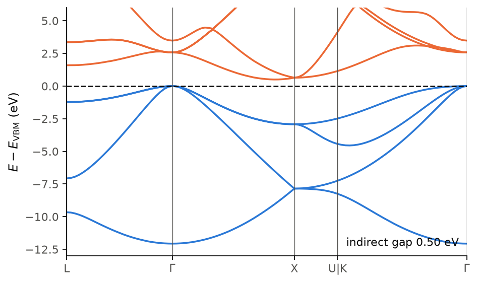
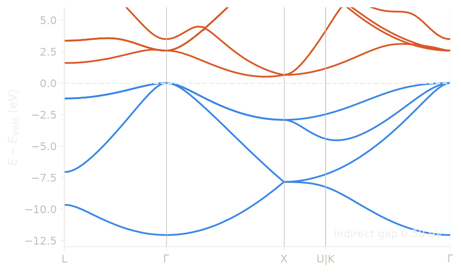
The figure shows silicon in LDA, with the four valence bands in blue and the four lowest conduction bands in orange. The zero is the top of the valence band, at \(\Gamma\), where three bands are degenerate. The bottom of the conduction band is on the line from \(\Gamma\) to X, at about 85% of the way to X, so the gap is indirect. Its value is 0.50 eV, while experiment gives 1.17 eV. This error comes from LDA and not from the code, since semilocal functionals underestimate band gaps. The degeneracies at \(\Gamma\), X and L are exact, because the density has the full symmetry of the crystal.

Code of this figure (docs/figures/bands_silicon/)

compute.py

"""The band structure of silicon along L-Gamma-X-U|K-Gamma."""
import numpy as np
from defuqumat import Calculator
from defuqumat.system.kpoints import KPoints
from common import PSEUDO, save

calc = Calculator.from_file("si.in", pseudo_dir=PSEUDO)
scf = calc.get_scf()

# the corners of the path, in units of 2 pi / a
corners = {"L": [0.5, 0.5, 0.5], "G": [0.0, 0.0, 0.0], "X": [1.0, 0.0, 0.0],
           "U": [1.0, 0.25, 0.25], "K": [0.75, 0.75, 0.0]}
labels = ["L", "G", "X", "U", "K", "G"]
counts = [26, 30, 10, 0, 32, 1]           # 0: a jump from U to K, which are equivalent
path = KPoints.band_path([corners[p] for p in labels], counts, calc.system.cell,
                         crystal=False)
bands = calc.get_bands(kpoints=path, nbnd=8)

vbm = bands.eigenvalues_ev[:, :4].max()
corner = np.cumsum([0] + [max(c, 1) for c in counts[:-1]])   # index of each corner
save(x=bands.path_length, energies=bands.eigenvalues_ev - vbm,
     ticks=bands.path_length[corner], labels=np.array(labels),
     gap=bands.gap(8), total_energy=scf.total_energy)

plot.py

"""The band structure of silicon: valence bands blue, conduction bands orange."""
import numpy as np
import style

d = np.load("data.npz")
names = {"G": r"$\Gamma$", "U": "U|K", "K": ""}


def draw():
    fig, ax = style.figure()
    e = d["energies"]
    for n in range(e.shape[1]):
        ax.plot(d["x"], e[:, n], color=style.color(0 if n < 4 else 1))
    ax.axhline(0.0, **style.reference())
    for t in d["ticks"]:
        ax.axvline(t, color=style.ink2(), lw=0.6)
    labels = [names.get(str(p), str(p)) for p in d["labels"]]
    keep = [i for i, p in enumerate(labels) if p]
    ax.set_xticks(d["ticks"][keep], [labels[i] for i in keep])
    ax.set_xlim(d["x"][0], d["x"][-1])
    ax.set_ylim(-13.0, 6.0)
    ax.set_ylabel(r"$E - E_{\rm VBM}$ (eV)")
    ax.text(0.98, 0.04, "indirect gap %.2f eV" % d["gap"], transform=ax.transAxes,
            ha="right")
    return fig


style.main(draw)

Band velocities

Let us now compute the band velocities. The group velocity of a Bloch state is the slope of its band:

\[ \mathbf v_{n\mathbf k} = \frac{1}{\hbar}\,\nabla_{\mathbf k}\,\varepsilon_{n\mathbf k} = \frac{1}{\hbar}\,\langle\psi_{n\mathbf k}|\,\nabla_{\mathbf k} H - \varepsilon_{n\mathbf k}\nabla_{\mathbf k} S\,|\psi_{n\mathbf k}\rangle . \]

The second form is the Hellmann-Feynman theorem, and \(S\) is the overlap operator, which is the identity for a norm-conserving pseudopotential. The code computes it with automatic differentiation of the Hamiltonian, and not by a finite difference of the bands. At the Fermi level this is the Fermi velocity, which enters the conductivity and the plasma frequency. We compute it with calc.get_band_velocities():

v = calc.get_band_velocities(kpoints=path, nbnd=8)
print(v.velocities.shape)   # (k-points, bands, 3), in Ry bohr

(41, 8, 3)

The unit is Ry bohr, with \(\hbar = 1\). If you do not pass kpoints, the velocities are on the k-points of the SCF.

Effective masses

Let us now go one derivative further, to the curvature of a band. Near a band edge a band is a parabola, and its curvature is the inverse effective mass tensor:

\[ \left(\frac{1}{m^*}\right)_{ab} = \frac{1}{2}\, \frac{\partial^2 \varepsilon_{n\mathbf k}}{\partial k_a\,\partial k_b} , \]

in units of \(1/m_e\), because \(\hbar^2/2m_e\) is exactly 1 Ry bohr\(^2\). The mass sets the mobility of the carriers and the density of states at the band edge, and cyclotron resonance measures it. The code takes the first derivative from the band velocity above and the second one from a small finite difference of the velocity around the k-point you give. We compute it with calc.get_effective_mass(), at the minimum of the conduction band of silicon:

import numpy as np

k = np.array([0.843, 0.0, 0.0])           # the minimum, in units of 2 pi / a
mass = calc.get_effective_mass(calc.system.cell.k_to_crystal(k), nbnd=8)
masses, axes = mass.principal(4)          # band 4, the lowest conduction band
print(np.round(masses, 3))                # in units of m_e
print(np.round(abs(axes[:, 0]), 3))       # the axis of the first mass

[0.952 0.19  0.19 ]
[1. 0. 0.]

The k-point is in crystal coordinates, so we convert it with cell.k_to_crystal(), and the tensor that comes back is cartesian. mass.inverse_mass has the shape (bands, 3, 3), mass.principal(n) gives the three masses of band \(n\) and their axes, and mass.density_of_states_mass(n) gives their geometric mean. Inside a degenerate multiplet a single band has no mass tensor, as for the velocity, so these bands are nan, and mass.multiplets holds the summed inverse mass of each multiplet, which is well defined.

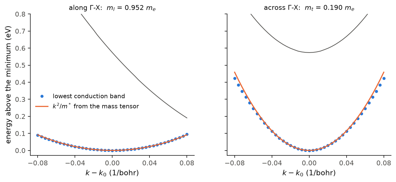
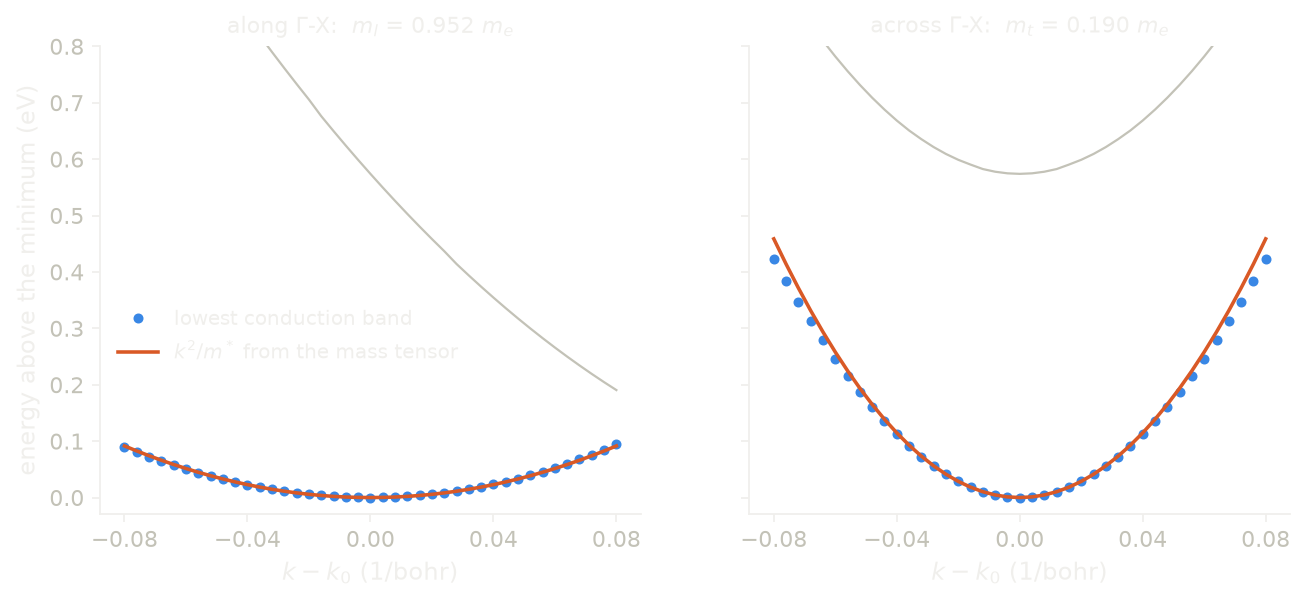
The minimum of the conduction band is on the line from \(\Gamma\) to X, at 0.843 of the way to X, and by symmetry there are six such valleys, one on each of the cubic axes. We see that each valley is a long ellipsoid. Along \(\Gamma\)-X the band is flat, with the longitudinal mass \(m_l = 0.952\,m_e\), and across it the band is steep, with the transverse mass \(m_t = 0.190\,m_e\). Cyclotron resonance gives 0.92 and 0.19 \(m_e\). The orange parabolas come only from the mass tensor at the minimum, while the blue points are a separate band calculation along the two lines. So the two agree near the minimum and move apart further out, where the band stops being quadratic: at 0.08 1/bohr across the valley the band is 0.036 eV below its parabola. The grey curve is the next conduction band. Along \(\Gamma\)-X it comes down and touches the lowest one at X, just outside the left panel. The finite difference is done at two step sizes and combined so that its leading error cancels, and mass.truncation gives the size of the part that was removed, 0.034 in units of \(1/m_e\) for this band.

Code of this figure (docs/figures/bands_masses/)

compute.py

"""The two effective masses of the conduction valley of silicon, against its bands."""
import numpy as np
from defuqumat import Calculator
from defuqumat.system.kpoints import KPoints
from defuqumat.units import RY_TO_EV
from common import PSEUDO, save

calc = Calculator.from_file("si.in", pseudo_dir=PSEUDO)
cell = calc.system.cell
band = 4                                       # the lowest conduction band

# the minimum of the band on the line from Gamma to X, in units of 2 pi / a
line = KPoints.band_path([[0.7, 0.0, 0.0], [1.0, 0.0, 0.0]], [60, 1], cell, crystal=False)
e = np.asarray(calc.get_bands(kpoints=line, nbnd=8).eigenvalues)[:, band]
i = np.argmin(e)
x = np.linspace(0.7, 1.0, 61)
x0 = x[i] - 0.005 * (e[i + 1] - e[i - 1]) / (2 * (e[i + 1] - 2 * e[i] + e[i - 1]))
k0 = np.array([x0, 0.0, 0.0])

# the mass tensor at the minimum, in 1/m_e, cartesian
mass = calc.get_effective_mass(np.asarray(cell.k_to_crystal(k0)), nbnd=8)
inverse = mass.inverse_mass[band]
print(f"minimum at {x0:.4f} of Gamma-X, m_l = {1 / inverse[0, 0]:.3f}, "
      f"m_t = {1 / inverse[1, 1]:.3f} m_e")

# the bands through the minimum, along [100] (longitudinal) and [010] (transverse)
t = np.linspace(-0.08, 0.08, 41)               # 1/bohr
cuts = []
for direction in ([1.0, 0.0, 0.0], [0.0, 1.0, 0.0]):
    ends = [k0 + t[0] / cell.tpiba * np.array(direction),
            k0 + t[-1] / cell.tpiba * np.array(direction)]
    cut = calc.get_bands(kpoints=KPoints.band_path(ends, [40, 1], cell, crystal=False),
                         nbnd=8)
    cuts.append(np.asarray(cut.eigenvalues)[:, band:] * RY_TO_EV)

e0 = mass.eigenvalues[band] * RY_TO_EV
save(t=t, longitudinal=cuts[0] - e0, transverse=cuts[1] - e0,
     inverse_mass=inverse, truncation=mass.truncation[band], x0=x0)

plot.py

"""The conduction valley of silicon along and across Gamma-X, with the two mass parabolas."""
import numpy as np
import style

d = np.load("data.npz")
t, inverse = d["t"], d["inverse_mass"]
ry_to_ev = 13.605693122994


def draw():
    fig, axs = style.figure(2, sharey=True)
    cuts = [(d["longitudinal"], inverse[0, 0], r"along $\Gamma$-X:  $m_l$"),
            (d["transverse"], inverse[1, 1], r"across $\Gamma$-X:  $m_t$")]
    for ax, (bands, curvature, name) in zip(axs, cuts):
        ax.plot(t, bands[:, 1:], color=style.ink2(), lw=1.0)
        ax.plot(t, bands[:, 0], "o", ms=3.5, color=style.color(0),
                label="lowest conduction band")
        ax.plot(t, curvature * t**2 * ry_to_ev, color=style.color(1),
                label=r"$k^2/m^*$ from the mass tensor")
        ax.set_title(name + f" = {1 / curvature:.3f} $m_e$", fontsize=10)
        ax.set_xlabel(r"$k - k_0$ (1/bohr)")
        ax.set_xticks([-0.08, -0.04, 0.0, 0.04, 0.08])
        ax.set_ylim(-0.03, 0.8)
    axs[0].set_ylabel("energy above the minimum (eV)")
    axs[0].legend(loc="center left", bbox_to_anchor=(0.0, 0.38))
    return fig


style.main(draw)

Limits

For a spin-polarized run (nspin = 2), bands.gap(nelec) needs the filling of each channel. You give it as bands.gap(nelec, tot_magnetization=m), or as bands.gap(occupied=(n_up, n_down)). Without one of them it gives an error. The gap is taken over both channels, so it can go from the top of one channel to the bottom of the other. bands.band_edges(...) gives the two levels.

Inside a degenerate multiplet a single band has no well-defined velocity. There, each row of v.velocities holds, for each direction, the slopes of the bands that the multiplet splits into, in ascending order, and v.degenerate_by_spin marks these rows.

get_effective_mass() gives an error on a spin spiral, because its stencil needs the bands at new k-points, and a spiral cannot yet move its two spheres to another k-list. The band velocities on the k-points of the SCF work. Two eigenvalues closer than degeneracy_tol = 1e-5 Ry at the k-point form a degenerate multiplet. Inside it a single band has no mass tensor, because the eigensolver can rotate the bands inside the multiplet. These bands are nan in mass.inverse_mass, mass.principal(n) gives an error for them, and mass.multiplets holds the summed inverse mass of the multiplet, which is invariant.

The step delta, 0.025 1/bohr by default, is the outermost point of the stencil with both method="velocity" and method="eigenvalue". The code does not tune it, and it reports the error that the two step sizes removed in mass.truncation.

The notebooks for this page are 02, silicon and 29, effective masses.