Dielectric constant, Born charges and phonons

In this page we compute how a crystal responds to a static electric field, to a displacement of its atoms and to a strain. These are second derivatives of the total energy: the dielectric constant, the Born effective charges, the phonons at the zone centre and at any wavevector, and, in a metal, the coupling of the phonons to the electrons, which gives the phonon linewidth.

The dielectric constant and the Born charges

We start with a uniform static field \(\boldsymbol{\mathcal E}\) on an insulator, with the ions held fixed. The electrons polarize, and the field also pushes on each ion. The two responses are

\[ \epsilon^{\infty}_{ij} = \delta_{ij} + 4\pi\,\frac{\partial P_i}{\partial \mathcal E_j}, \qquad Z^{\ast}_{I,ij} = \frac{\partial F_{Ij}}{\partial \mathcal E_i} = \Omega\,\frac{\partial P_i}{\partial u_{Ij}} , \]

meaning that \(\epsilon^\infty\) is the screening of the field by the electrons alone, and the Born charge \(Z^\ast\) of atom \(I\) is both the force that the field puts on the atom and the dipole that the atom carries when it moves. \(Z^\ast\) is in units of the electron charge. The refractive index far above the phonon frequencies is \(n = \sqrt{\epsilon^\infty}\), which is what ellipsometry measures, and \(Z^\ast\) is what makes an optical phonon infrared-active and what splits the longitudinal and transverse optical modes of a polar crystal.

Both come from the first-order change of the occupied states, which we compute from the Sternheimer equation,

\[ \big(\hat H - \varepsilon_n \hat S + \alpha \hat Q\big)\,|\Delta\psi_n\rangle = -\hat P_c^{\dagger}\,\Delta V\,|\psi_n\rangle , \]

a linear equation for each occupied band, so we need no empty states and we never divide by \(\varepsilon_n - \varepsilon_m\). \(\Delta V\) contains the change of the Hartree and exchange-correlation potential, so the equation is solved self-consistently, the same way as the SCF. Here we take AlAs, where the two atoms are different, and we compute it with alas.get_dielectric_tensor():

import numpy as np
from defuqumat import Calculator

alas = Calculator.from_file("docs/figures/phonons_silicon_q/alas.in",
                            pseudo_dir="tests/data/pseudo")
eps = alas.get_dielectric_tensor()
print(np.round(eps.epsilon, 4))
print("Z* of Al:")
print(np.round(eps.born_charges[0], 4))
print("Z*_xx of Al and As:", np.round(eps.born_charges[:, 0, 0], 4))
print(f"sum over the cell: {eps.born_charges[:, 0, 0].sum():.4f}")

[[ 9.5203  0.     -0.    ]
 [-0.      9.5203 -0.    ]
 [ 0.     -0.      9.5203]]
Z* of Al:
[[2.1011 0.     0.    ]
 [0.     2.1011 0.    ]
 [0.     0.     2.1011]]
Z*_xx of Al and As: [ 2.1011 -2.1658]
sum over the cell: -0.0648

eps.epsilon is the \(3\times3\) tensor in Cartesian axes, and eps.isotropic is its trace over three. The Born charges come from the same solve, so eps.born_charges has them, with the shape (atoms, 3, 3). alas.get_born_charges() returns only this array. In the cubic zincblende structure both tensors are diagonal with three equal elements, as we see, so this calculation gives \(\epsilon^\infty = 9.52\) for AlAs, and the charges \(+2.10\) on Al and \(-2.17\) on As. The \(4\times4\times4\) mesh and the cutoff of 25 Ry are small, so \(\epsilon^\infty\) is not converged, and you check it on a denser k-mesh. These are far from the nominal charges \(\pm 3\) of a fully ionic picture, which is what a covalent bond with some ionic character gives. A uniform displacement of the whole crystal carries no dipole, so the Born charges of the cell must add up to zero, which is the charge neutrality sum rule. Here they add up to \(-0.065\), which is the error of this small calculation, with a \(4\times4\times4\) mesh and 25 Ry. The sum is a free check of convergence, so print it for your own crystal.

Phonons at the zone centre

Let us now move the atoms. The force constants are the second derivatives of the energy with respect to the displacements \(u_{I\alpha}\), and the phonon frequencies are the eigenvalues of the force constants divided by the masses:

\[ C_{I\alpha,J\beta} = \frac{\partial^2 E}{\partial u_{I\alpha}\,\partial u_{J\beta}}, \qquad \sum_{J\beta} \frac{C_{I\alpha,J\beta}}{\sqrt{M_I M_J}}\, e_{J\beta} = \omega^2\, e_{I\alpha} . \]

When an atom moves, the electrons follow it, and this is again the Sternheimer equation, now with the change of the pseudopotential as the perturbation. At the zone centre the optical modes are what Raman and infrared spectroscopy measure. We compute them with silicon.get_phonons():

silicon = Calculator.from_file("docs/figures/phonons_silicon_q/si.in",
                               pseudo_dir="tests/data/pseudo")
gamma = silicon.get_phonons()
print(np.round(gamma.frequencies, 2), "cm^-1")
print(f"acoustic residue {gamma.acoustic_residue:.2f} cm^-1")
print(gamma.matrix.shape)

[  4.33   4.33   4.33 519.2  519.2  519.2 ] cm^-1
acoustic residue 4.33 cm^-1
(2, 3, 2, 3)

gamma.frequencies is in cm\(^{-1}\), from low to high, and gamma.eigenvectors holds the modes as columns. An unstable mode has \(\omega^2 < 0\), and it comes as a negative frequency. gamma.matrix is the force constant matrix in Ry/bohr\(^2\), with the shape (atom, direction, atom, direction).

We see the triply degenerate optical mode of silicon at 519.20 cm\(^{-1}\), which is the Raman line. The three acoustic modes, a rigid translation of the crystal, must be at zero frequency exactly, and here they are at 4.33 cm\(^{-1}\). gamma.acoustic_residue gives this number. It comes from the finite plane-wave basis, because the energy changes a little when the atoms move relative to the FFT grid, so the crystal is not exactly invariant under a translation, and a larger ecutrho makes it smaller. We checked this number in an independent way. We moved the whole crystal by a small step and took the second derivative of the energy by finite differences, and this gives 4.33 cm\(^{-1}\) too.

The response loop of get_phonons() stops at tr2 = 1e-18, which is tighter than the tr2_ph = 1e-14 of ph.x. If you want the stop of ph.x, for example to compare with it number by number, you pass tr2=1e-14. Then the residue on this cell is 5.68 cm\(^{-1}\), so about 1.4 cm\(^{-1}\) of it is the loop that stops early, while the optical mode moves by only 0.0015 cm\(^{-1}\). The tighter default costs 9 passes of the loop instead of 6. We do not correct the residue by default, so you see how large it is, and acoustic_sum_rule=True removes it from the matrix by hand.

Phonons at any wavevector

Away from the zone centre, the atoms move with a phase from one cell to the next, \(u_{I\alpha}(\mathbf R) = u_{I\alpha}\,e^{i\mathbf q\cdot\mathbf R}\), and the force constants become the dynamical matrix

\[ D_{I\alpha,J\beta}(\mathbf q) = \frac{1}{\sqrt{M_I M_J}} \sum_{\mathbf R} C_{I\alpha,J\beta}(\mathbf R)\, e^{-i\mathbf q\cdot\mathbf R}, \]

a complex Hermitian matrix of size \(3n_{\rm at}\) whose eigenvalues are \(\omega^2_{\mathbf q\nu}\). A perturbation with wavevector \(\mathbf q\) couples a state at \(\mathbf k\) to a state at \(\mathbf k+\mathbf q\), so we solve the Sternheimer equation for this pair, with no supercell. The phonon dispersion is what inelastic neutron and x-ray scattering measure. We compute one wavevector with silicon.get_phonons_at_q(q=...). Here q is in Cartesian units of \(2\pi/a\) with q_cartesian=True, and in crystal coordinates of the reciprocal lattice if you do not give it:

for name, q in [("X", (1, 0, 0)), ("L", (0.5, 0.5, 0.5))]:
    phonon = silicon.get_phonons_at_q(q=q, q_cartesian=True)
    print(name, np.round(phonon.frequencies, 2))
print(phonon.matrix.shape, phonon.matrix.dtype)

X [132.8  132.8  405.32 405.32 455.12 455.12]
L [101.79 101.79 382.24 405.1  488.03 488.03]
(2, 3, 2, 3) complex128

At X the two transverse acoustic modes are at 132.80 cm\(^{-1}\), the longitudinal acoustic and longitudinal optical modes meet at 405.32 cm\(^{-1}\), which the diamond structure forces at this point, and the two transverse optical modes are at 455.12 cm\(^{-1}\). At L all four branches are apart, with the transverse ones doubly degenerate: 101.79, 382.24, 405.10 and 488.03 cm\(^{-1}\). phonon.matrix is the force constant matrix at \(\mathbf q\), \(\sum_{\mathbf R} C(\mathbf R)\, e^{-i\mathbf q\cdot\mathbf R}\), in Ry/bohr\(^2\) and without the masses, with the shape (atom, direction, atom, direction). It has complex elements because of the phase \(e^{-i\mathbf q\cdot\mathbf R}\), and the masses enter only when it is diagonalised. Each q is a full calculation of its own, which here is about 30 s on one core.

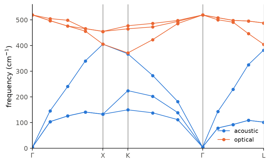
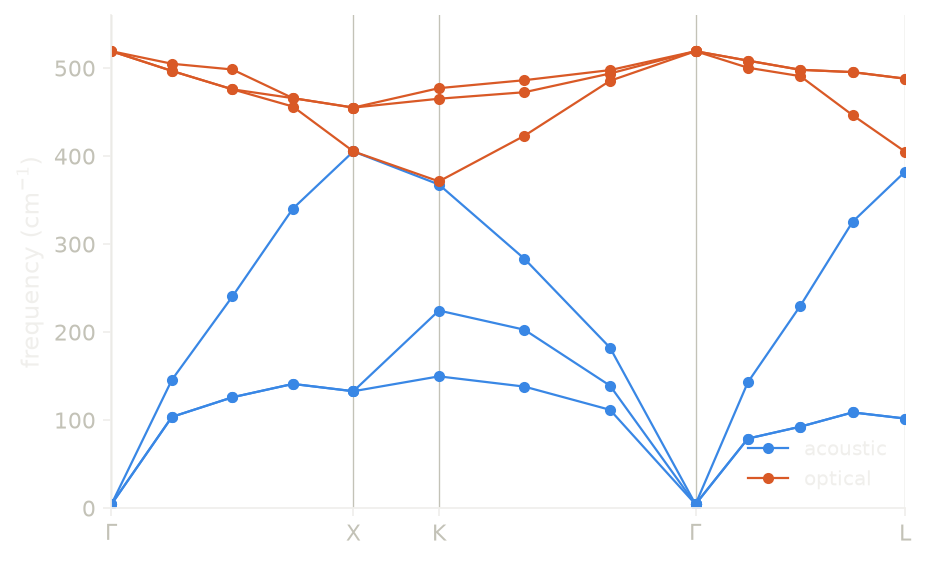
Here we computed the six branches of silicon at 13 wavevectors along \(\Gamma\)-X-K-\(\Gamma\)-L, on the same \(4\times4\times4\) mesh, in 422 s on one core. Each dot is one call of get_phonons_at_q, and the lines only join the dots, since the code does not interpolate the force constants between wavevectors. The segment from X to K starts at \((1,1,0)\,2\pi/a\), which is the same point as X shifted by a reciprocal lattice vector, and the two give the same six frequencies to the last printed digit. Along \(\Gamma\)-X and \(\Gamma\)-L the transverse branches stay degenerate, while along K-\(\Gamma\) the symmetry is lower and all six branches split. The upper three branches stay between 371 and 519 cm\(^{-1}\), and the longitudinal acoustic branch rises to 405 cm\(^{-1}\) at X. At \(\Gamma\) the acoustic branches start at 4.4 cm\(^{-1}\) rather than at zero. This is the same error as above. get_phonons_at_q stops its response loop a little earlier than get_phonons() does, so its residue of 4.37 cm\(^{-1}\) is close to, but not exactly, the 4.33 cm\(^{-1}\) of get_phonons().

Code of this figure (docs/figures/phonons_silicon_q/)

compute.py

"""The phonon branches of silicon along Gamma-X-K-Gamma-L, one q at a time."""
import numpy as np
from defuqumat import Calculator
from common import PSEUDO, save

calc = Calculator.from_file("si.in", pseudo_dir=PSEUDO)

# q in units of 2 pi / a. X = (1, 1, 0) is the same point as X = (1, 0, 0),
# so the second segment goes from X to K along (1, 1, 0) and back to Gamma.
segments = [
    [(0, 0, 0), (0.25, 0, 0), (0.5, 0, 0), (0.75, 0, 0), (1, 0, 0)],
    [(1, 1, 0), (0.75, 0.75, 0), (0.5, 0.5, 0), (0.25, 0.25, 0), (0, 0, 0)],
    [(0, 0, 0), (0.125, 0.125, 0.125), (0.25, 0.25, 0.25), (0.375, 0.375, 0.375),
     (0.5, 0.5, 0.5)],
]
done = {}
x, frequencies, start = [], [], 0.0
for points in segments:
    for q in points:
        if q not in done:
            done[q] = calc.get_phonons_at_q(q=q, q_cartesian=True).frequencies
        x.append(start + np.linalg.norm(np.subtract(q, points[0])))
        frequencies.append(done[q])
    start = x[-1]

save(x=np.array(x), frequencies=np.array(frequencies),
     ticks=np.array([0.0, x[4], x[6], x[9], x[-1]]))

plot.py

"""The six phonon branches of silicon, one point per computed q."""
import numpy as np
import style

d = np.load("data.npz")
labels = [r"$\Gamma$", "X", "K", r"$\Gamma$", "L"]


def draw():
    fig, ax = style.figure()
    for t in d["ticks"]:
        ax.axvline(t, color=style.ink2(), lw=0.6)
    for n in range(d["frequencies"].shape[1]):
        ax.plot(d["x"], d["frequencies"][:, n], "-o", color=style.color(0 if n < 3 else 1),
                lw=1.0, ms=4)
    ax.plot([], [], "-o", color=style.color(0), lw=1.0, ms=4, label="acoustic")
    ax.plot([], [], "-o", color=style.color(1), lw=1.0, ms=4, label="optical")
    ax.set_xticks(d["ticks"], labels)
    ax.set_xlim(d["x"][0], d["x"][-1])
    ax.set_ylim(0.0, 560.0)
    ax.set_ylabel(r"frequency (cm$^{-1}$)")
    ax.legend(loc="lower right")
    return fig


style.main(draw)

Electron-phonon coupling in a metal

In a metal a phonon can decay into an electron-hole pair at the Fermi surface, so it has a finite lifetime. Its linewidth is

\[ \gamma_{\mathbf q\nu} = \frac{\pi}{2} \sum_{\mathbf k} w_{\mathbf k} \sum_{mn} \big|\mathbf z_{\nu}\cdot\mathbf g_{mn}(\mathbf k,\mathbf q)\big|^2\, \delta(\varepsilon_{n\mathbf k} - E_F)\,\delta(\varepsilon_{m\mathbf k+\mathbf q} - E_F), \qquad \lambda_{\mathbf q\nu} = \frac{\gamma_{\mathbf q\nu}}{\pi N(E_F)\,\omega_{\mathbf q\nu}^2}, \]

where \(g^{I\alpha}_{mn}(\mathbf k,\mathbf q) = \langle\psi_{m\mathbf k+\mathbf q}|\partial V/\partial u_{I\alpha}|\psi_{n\mathbf k}\rangle\) is the matrix element of the self-consistent change of the potential when atom \(I\) moves along \(\alpha\), the same \(\Delta V\) that the phonon at \(\mathbf q\) gives, and \(\mathbf z_\nu\) is the displacement pattern of mode \(\nu\). So the linewidth counts the pairs of states on the Fermi surface that are joined by \(\mathbf q\), weighted by how strongly the mode scatters them, and \(\lambda_{\mathbf q\nu}\) is the same coupling made dimensionless. The linewidth is measured by inelastic neutron or x-ray scattering, and the average of \(\lambda\) over the zone enters the superconducting \(T_c\). The two delta functions are broadened by Gaussians, and the code returns the result for a list of broadenings \(\sigma\), which is how you see whether it is converged. Here we take fcc aluminium, and we compute it with aluminium.get_electron_phonon(q=...):

aluminium = Calculator.from_file("docs/figures/phonons_linewidth/al.in",
                                 pseudo_dir="tests/data/pseudo")
el = aluminium.get_electron_phonon(q=(0.5, 0, 0), q_cartesian=True)
print("frequencies", np.round(el.frequencies, 2), "cm^-1")
for i in (0, 2, 4, 9):
    print(f"sigma {el.sigmas[i]:.2f} Ry   N(E_F) {el.dos[i]:.3f}   "
          f"gamma {np.round(el.gamma_ghz[i], 2)} GHz   lambda {np.round(el.lambdas[i], 3)}")

frequencies [140.08 140.08 216.46] cm^-1
sigma 0.02 Ry   N(E_F) 2.676   gamma [0.   0.   6.46] GHz   lambda [0.   0.   0.06]
sigma 0.06 Ry   N(E_F) 2.782   gamma [ 4.6   4.6  31.81] GHz   lambda [0.098 0.098 0.284]
sigma 0.10 Ry   N(E_F) 2.781   gamma [ 6.82  6.82 30.65] GHz   lambda [0.146 0.146 0.274]
sigma 0.20 Ry   N(E_F) 2.674   gamma [ 7.32  7.32 29.3 ] GHz   lambda [0.162 0.162 0.272]

el.sigmas is the list of broadenings, from 0.02 to 0.20 Ry, and every other array has one row per broadening: el.gamma_ghz the linewidth of each mode in GHz (el.gamma in Ry), el.lambdas the coupling \(\lambda_{\mathbf q\nu}\), and el.dos the density of states at the Fermi level, in states per spin per Ry per cell. el.phonons is the phonon at \(\mathbf q\) that the coupling was computed with.

At \(\mathbf q = (1/2, 0, 0)\,2\pi/a\), halfway to X, the two transverse modes are at 140.08 cm\(^{-1}\) and the longitudinal one at 216.46 cm\(^{-1}\). At the smallest broadening, 0.02 Ry, the mesh finds only a few pairs of states at the Fermi level. These few pairs give the longitudinal mode 6.46 GHz, a fifth of its converged value, and the transverse modes almost nothing (0.0002 GHz). So 0.02 Ry is too small for the \(8\times8\times8\) mesh, and this is not physics. From 0.06 Ry the longitudinal linewidth stays near 30 GHz (31.81, 30.65 and 29.30 GHz) and its \(\lambda\) near 0.28, while the transverse one still grows from 4.6 to 7.3 GHz. A linewidth of 30 GHz is 1 cm\(^{-1}\), so the longitudinal mode is sharp, with a width of 0.5 per cent of its frequency.

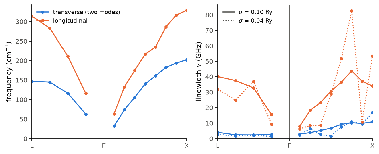
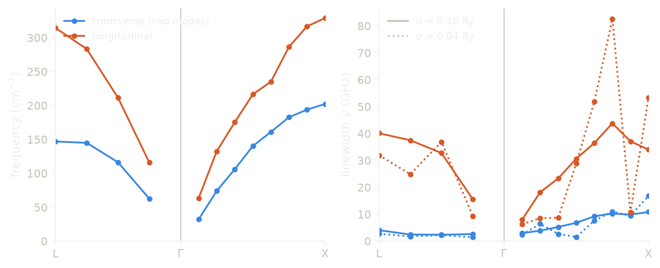
Here we computed the coupling at 12 wavevectors from L to X on the \(8\times8\times8\) mesh, in 485 s on one core. \(\Gamma\) itself is missing, because the coupling at \(\mathbf q = 0\) gives an error: its acoustic modes have zero frequency, and we have no reference for it. For the phonons at the zone centre you use get_phonons(). On the left we see the branches, which go from 147 and 314 cm\(^{-1}\) at L to 202 and 329 cm\(^{-1}\) at X. On the right we see the linewidths, at \(\sigma = 0.10\) Ry (solid) and 0.04 Ry (dotted). The longitudinal mode couples much more than the transverse ones, with a linewidth up to 44 GHz while the transverse ones stay below 11 GHz, because it compresses the crystal and so changes the potential that the electrons feel. The dotted curve jumps from point to point, from 82.6 GHz at \((0.75, 0, 0)\) to 10.7 GHz at the next point, so at 0.04 Ry this mesh does not sample the Fermi surface and the solid curve is the one to read.

We checked this mesh by running three wavevectors again on a \(12\times12\times12\) mesh. At \(\sigma = 0.10\) Ry the longitudinal linewidth moves little: 30.65 to 30.46 GHz at \((0.5, 0, 0)\) and 36.47 to 35.73 GHz at \((0.625, 0, 0)\). The frequencies move more, and they are not converged on the \(8\times8\times8\) mesh. The longitudinal mode goes from 216.46 to 226.28 cm\(^{-1}\) at \((0.5, 0, 0)\) and from 234.99 to 257.93 cm\(^{-1}\) at \((0.625, 0, 0)\), so the kink of the longitudinal branch at that point in the figure comes from the mesh. Near \(\Gamma\), at \((0.125, 0, 0)\), the transverse mode goes from 32.13 to 38.54 cm\(^{-1}\), which is 20 per cent. For a real metal you check the mesh and the smearing degauss of the SCF together, since both set the Fermi surface.

Code of this figure (docs/figures/phonons_linewidth/)

compute.py

"""The phonons of aluminium and their electron-phonon linewidths, along L-Gamma-X."""
import numpy as np
from defuqumat import Calculator
from common import PSEUDO, save

calc = Calculator.from_file("al.in", pseudo_dir=PSEUDO)

# q in units of 2 pi / a. A metal at q = 0 gives an error, so Gamma is left out.
to_l = [(t, t, t) for t in (0.5, 0.375, 0.25, 0.125)]
to_x = [(t, 0, 0) for t in (0.125, 0.25, 0.375, 0.5, 0.625, 0.75, 0.875, 1.0)]
results = [calc.get_electron_phonon(q=q, q_cartesian=True) for q in to_l + to_x]

save(x=np.array([-np.linalg.norm(q) for q in to_l] + [q[0] for q in to_x]),
     frequencies=np.array([r.frequencies for r in results]),
     gamma_ghz=np.array([r.gamma_ghz for r in results]),    # (q, sigma, mode)
     lambdas=np.array([r.lambdas for r in results]),
     sigmas=results[0].sigmas, dos=results[0].dos)

plot.py

"""The phonons of aluminium and their linewidths, along L-Gamma-X."""
import numpy as np
import style

d = np.load("data.npz")
SIGMA = 4                       # the broadening shown, d["sigmas"][SIGMA] in Ry
modes = {0: "transverse (two modes)", 2: "longitudinal"}


def draw():
    fig, (a, b) = style.figure(2)
    for k, (mode, name) in enumerate(modes.items()):
        a.plot(d["x"][:4], d["frequencies"][:4, mode], "-o", color=style.color(k), ms=4)
        a.plot(d["x"][4:], d["frequencies"][4:, mode], "-o", color=style.color(k), ms=4,
               label=name)
        for s, ls in ((1, ":"), (SIGMA, "-")):
            g = d["gamma_ghz"][:, s, mode]
            b.plot(d["x"][:4], g[:4], ls, marker="o", color=style.color(k), ms=4)
            b.plot(d["x"][4:], g[4:], ls, marker="o", color=style.color(k), ms=4)
    b.plot([], [], "-", color=style.ink2(), label=r"$\sigma$ = %.2f Ry" % d["sigmas"][SIGMA])
    b.plot([], [], ":", color=style.ink2(), label=r"$\sigma$ = %.2f Ry" % d["sigmas"][1])
    for ax in (a, b):
        style.zero_line(ax, vertical=True)
        ax.set_xticks([d["x"][0], 0.0, d["x"][-1]], ["L", r"$\Gamma$", "X"])
        ax.set_xlim(d["x"][0], d["x"][-1])
        ax.set_ylim(bottom=0.0)
    a.set_ylabel(r"frequency (cm$^{-1}$)")
    b.set_ylabel(r"linewidth $\gamma$ (GHz)")
    a.legend(loc="upper left")
    b.legend(loc="upper left")
    return fig


style.main(draw)

The response to a strain

The third perturbation is a homogeneous strain \(\varepsilon_{ij}\), which deforms the cell and carries the atoms with it. Its first-order response is the change of the occupied states and of the density, \(\partial\psi/\partial\varepsilon_{ij}\) and \(\partial n/\partial\varepsilon_{ij}\), and the change of the band energies,

\[ \Xi_{n\mathbf k,ij} = \frac{\partial \varepsilon_{n\mathbf k}}{\partial \varepsilon_{ij}} , \]

which are the deformation potentials, meaning how far a strain moves each band. They are what optical absorption and photoluminescence under pressure measure. A deformation potential of one band alone has no meaning in a periodic solid, because the average electrostatic potential of the crystal is not defined, so only the difference between two bands is a physical number. We compute the response with silicon.get_strain_response(), and here we take the change of the valence band width at \(\Gamma\), from the lowest band to the top triplet, under a uniform strain \(e\) along all three axes:

strain = silicon.get_strain_response()
d = strain.deigenvalues[:, :, 0, 0]          # spin 0, k = Gamma, in Ry
hydro = d[0, 0] + d[1, 1] + d[2, 2]          # a uniform strain e on all three axes
width = (hydro[1:4].mean() - hydro[0]) * 13.6057
print(strain.converged, strain.deigenvalues.shape)
print(f"d(valence band width)/de at Gamma: {width:.2f} eV")

True (3, 3, 1, 64, 4)
d(valence band width)/de at Gamma: -20.93 eV

strain.deigenvalues has the shape (3, 3, spin, k-point, occupied band), in Ry per unit strain, and the first k-point of this unshifted mesh is \(\Gamma\). Only the occupied bands are in it, so a band gap deformation potential is not available this way. The valence band of silicon is 12.08 eV wide at \(\Gamma\), and it gets narrower as the crystal expands, by 20.93 eV per unit \(e\). As a reference, a free-electron band has a width proportional to \(V^{-2/3}\), which gives \(-2 \times 12.08 = -24.2\) eV, so the valence band of silicon follows the free-electron picture roughly. In the degenerate top triplet we take the average of the three bands, since the single values inside a degenerate set depend on the basis chosen in it. The same response gives the clamped-ion elastic constants, which we compute in the page about stress with get_elastic_constants().

Limits

The dielectric constant and the Born charges are for insulators, and a metal gives an error, because \(\epsilon^\infty\) is not defined there. They work for nspin = 2. A noncollinear or spin-orbit run works with norm-conserving, ultrasoft and PAW datasets if it has no net magnetization, and a noncollinear run with a magnetization gives an error.

Every response gives an error for a ground state converged with a magnetic field or a constrained moment, because the field the ground state converged under is not the one in the input, so you run the ground state again without them. It also gives an error for a Hubbard \(U\) and for a potential-only meta-GGA (tb09, bj06), which has no total energy to differentiate. For a metal the response needs a smearing, so tetrahedra and occupations = 'from_input' give an error.

In a spin-polarized or noncollinear run with fixed occupations, every response gives an error when the filling cuts a degenerate multiplet, meaning that the gap to the first empty band is below \(10^{-5}\) Ry, as in an atom with Hund's rule. Which member of the multiplet is occupied is then arbitrary, so you occupy the whole shell or use a smearing. tot_magnetization with a smearing gives an error, because the two spin channels then have two Fermi levels. The screened response of a magnetic system with vacuum gives an error for a GGA, because the exchange-correlation kernel is infinite where one spin channel is empty, and with the LDA it works.

The phonons, the Raman tensors, the strain response, the elastic constants and the electrostriction tensors give an error for a noncollinear or spin-orbit run. The Raman tensors, the strain response, the elastic constants and the electrostriction tensors also give an error for nspin = 2. The phonons at \(\Gamma\) work for nspin = 2. They give an error there only when the run walks the k-points in chunks. This is memory_mode = 'memory', which is the default on a GPU, and a streamed store. On a CPU the default memory_mode = 'speed' works. The phonons at \(\Gamma\) of an ultrasoft or PAW metal give an error.

The static \(\chi^{(2)}\) and the electro-optic tensor from this response give an error, because the term \(\langle u_i|r_k|u_j\rangle\), where the field sits between two first-order states, has nothing to build it from. The Raman tensors do not need this term and they work.

The phonons at \(\mathbf q\) need the whole k-mesh, so without nosym they give an error, because the response would have to be averaged over the small group of \(\mathbf q\), which is not the group of the crystal. We run them with noinv as well and on an unshifted mesh, which is the mesh that is closed under the point group. They give an error for ultrasoft and PAW datasets, for a GGA functional such as PBE, for spinors, spin spirals, DFT+U and nosource, and for a potential-only meta-GGA (tb09, bj06), as every response does. A norm-conserving dataset with a nonlinear core correction works. The GGA error is there with and without spin, because with a GGA the result at \(\mathbf q\) was wrong by tens of cm\(^{-1}\), so you use an LDA functional. With the LDA they work for nspin = 2 in an insulator, which we checked on a magnetic hydrogen chain against the same chain doubled, at \(\Gamma\). A spin-polarized metal gives an error, and so does nspin = 2 together with a nonlinear core correction, because we have not checked the two together. With nspin = 2 they also give an error when the run walks the k-points in chunks, as the phonons at \(\Gamma\) do, and the electron-phonon coupling works only for nspin = 1. For a metal they work at \(\mathbf q = 0\), where the Fermi level moves and the code moves it as ph.x does. At a reciprocal lattice vector other than zero they give an error, and you use \(\mathbf q = 0\) instead. On the k-chunked route, which a GPU takes in memory_mode = 'memory', a metal at \(\mathbf q = 0\) gives an error, and you use get_phonons(). There is no interpolation of the force constants, so a dispersion is one calculation per wavevector.

With nosym, the dielectric constant, the Born charges, the phonons at \(\Gamma\), the Raman tensors, the strain response and the electrostriction tensors need an unshifted k-mesh, and a shifted one gives an error, because a shifted mesh does not have the symmetry of the crystal.

With symmetry, the phonons of a part of the atoms (atoms=) need a set of atoms that the symmetry operations map onto itself. For another set you get an error, and it names the smallest such set that contains yours. With nosym any set works. On a GPU in memory_mode = 'memory', or with a streamed wavefunction store, a part of the atoms with symmetry also gives an error. Use nosym there, or a memory mode that holds the whole k-mesh. You can also get the phonons of a part of the atoms from the response that the Raman tensors keep (keep_internals=True). With nosym this works on the k-chunked route too.

The electron-phonon coupling gives an error for an insulator, where there are no states at the Fermi level, at \(\mathbf q = 0\), and for everything that the phonons at \(\mathbf q\) refuse. There is no Eliashberg function \(\alpha^2F(\omega)\), no \(\lambda\) averaged over the zone and no \(T_c\).

The strain response is for an insulator with nspin = 1, and it is clamped-ion. It works with norm-conserving, ultrasoft and PAW datasets, but the elastic constants need a norm-conserving dataset and the whole k-mesh.

The notebooks for this page are 19, linear response, 20, phonons and 49, electron-phonon coupling.