Spin spirals¶

In this page we compute flat spin spirals of any wavevector in one unit cell. We compute the energy \(E(\mathbf q)\) as a function of the wavevector, we relax the wavevector, and we compute the Dzyaloshinskii-Moriya energy, the energy that tells a spiral from its mirror image.

The generalized Bloch theorem¶

We start with what a spiral does to the periodicity. A flat spiral turns the moment by \(\mathbf q\cdot\mathbf R\) from one cell to the next. For a general \(\mathbf q\) it is not periodic, so a supercell would have to be very large. Without spin-orbit coupling there is a way around this. In a frame that turns with the spins, the density and the potential are periodic again, so the two spinor components carry Bloch phases that differ by \(\mathbf q\):

\[ \psi_{n\mathbf k}(\mathbf r) = e^{i\mathbf k\cdot\mathbf r} \begin{pmatrix} e^{-i\mathbf q\cdot\mathbf r/2}\; u^{\uparrow}_{n\mathbf k}(\mathbf r) \\[3pt] e^{+i\mathbf q\cdot\mathbf r/2}\; u^{\downarrow}_{n\mathbf k}(\mathbf r) \end{pmatrix} . \]

This is the generalized Bloch theorem. The up component lives at \(\mathbf k + \mathbf q/2\) and the down component at \(\mathbf k - \mathbf q/2\), each on its own plane-wave sphere, meaning that any \(\mathbf q\) is a calculation in one cell. You set it with spiral_q(1:3) in &system, in crystal units of the reciprocal lattice vectors (vqlss in Elk). pw.x has no spin spiral. Neutron diffraction sees a spiral as magnetic satellites at \(\pm\mathbf q\) around the Bragg peaks.

import numpy as np
from defuqumat import Calculator

chain = Calculator.from_file("docs/figures/spirals_eq/h-chain.in",
                             pseudo_dir="tests/data/pseudo")
scf = chain.get_scf()
print(f"q = {chain.system.spiral_q}, E = {scf.total_energy:.8f} Ry")
print(f"|m| = {np.linalg.norm(scf.magnetization_vector):.4f} mu_B per cell")

q = (0.0, 0.0, 0.25), E = -0.95474611 Ry
|m| = 0.5397 mu_B per cell

Here we take a chain of hydrogen atoms along \(z\), with one atom per cell, and the moment turns by a quarter turn per cell. In the turning frame this is a normal SCF. The moment of the cell depends on the frame, so only the energy and the size of the moment are physical.

The gradient correction of a turning moment¶

We now ask what a gradient functional such as PBE does with a moment that turns. The answer of pw.x, which is noncollinear_gga = 'kubler' here, is to evaluate the collinear functional on \((n\pm|\mathbf m|)/2\). On a spiral \(|\mathbf m|\) has a kink at every node of \(\mathbf m\), so its gradient diverges there and the SCF needs many iterations. With noncollinear_gga = 'grad_m' in &system, the default for every noncollinear magnetic run with a gradient or meta-GGA functional, we build exchange from the gradients of the components of \(\mathbf m\) instead, meaning that it is the collinear exchange wherever \(\nabla\mathbf m\) is parallel to \(\mathbf m\) and it is smooth where \(\mathbf m\) vanishes. On a spiral this gradient carries \(\mathbf q\), so it also enters \(dE/d\mathbf q\). The two choices are one functional on a collinear state and differ on a canted or spiral one, so when you compare such a state with pw.x or Elk you set noncollinear_gga = 'kubler'.

E(q) and its slope¶

Let us now compute the energy as a function of \(\mathbf q\). We do this with get_spiral_scan(wavevectors), which runs one SCF for each \(\mathbf q\). The curve \(E(\mathbf q)\) is the frozen-magnon dispersion. Its shape near \(\mathbf q = 0\) gives the spin stiffness, and a fit of a Heisenberg model to it gives the exchange constants \(J_{ij}\). With gradients=True the scan also computes \(dE/d\mathbf q\) at each point, by automatic differentiation at fixed wavefunctions, as we do for a force.

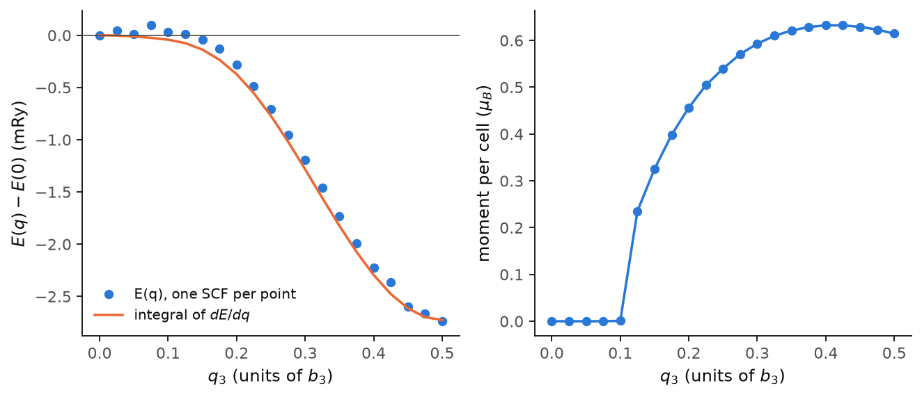
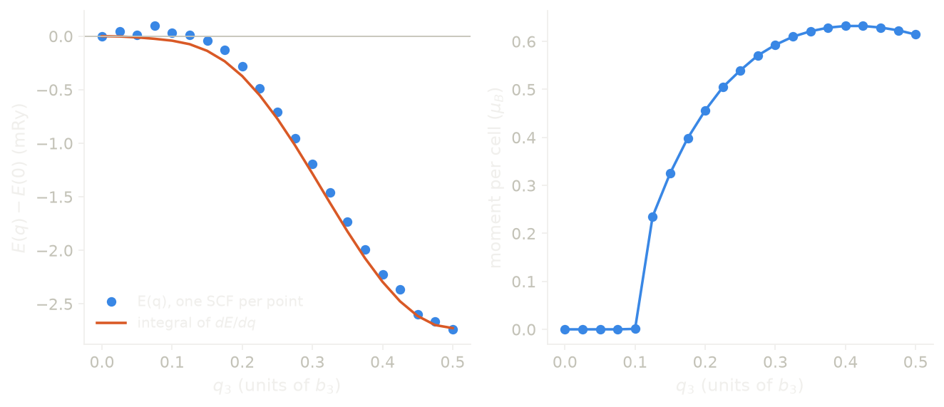
E(q) of the hydrogen chain from the energies and from the slope, and the size of the moment.

In the left panel we see \(E(q)\) for 21 wavevectors along the chain. The points are the energies of the SCF runs, and the line is the integral of the slope \(dE/dq\) along the scan. Both fall to \(-2.73\) mRy at the zone boundary, \(q = 1/2\), so the ground state of the chain is the antiferromagnet. The two agree to 0.12 mRy. The points are not monotonic at small \(q\), while the integral is. The reason is that the plane-wave basis is built again at each \(q\), so each energy has a small step whenever a plane wave crosses the cutoff. The slope is taken in a fixed basis and has no such steps. The right panel shows why the curve is flat at small \(q\): below \(q \approx 0.1\) the chain has no moment at all. A slow spiral costs more than the polarization gains, so the SCF finds the nonmagnetic state there.

Code of this figure (docs/figures/spirals_eq/)

compute.py

"""E(q) of the hydrogen chain, from the energies and from the slope dE/dq."""
import numpy as np
from defuqumat import Calculator
from common import PSEUDO, save

chain = Calculator.from_file("h-chain.in", pseudo_dir=PSEUDO)
q = np.linspace(0.0, 0.5, 21)
scan = chain.get_spiral_scan([[0.0, 0.0, x] for x in q], gradients=True,
                             max_iterations=200)

save(q=q, direct=scan.relative, integrated=scan.integrated,
     moment=np.linalg.norm(scan.moments, axis=1), converged=np.asarray(scan.converged))

plot.py

"""E(q) of the chain two ways, and the size of the moment along the curve."""
import numpy as np
import style

d = np.load("data.npz")


def draw():
    fig, (a, b) = style.figure(2)
    a.plot(d["q"], d["direct"], "o", label="E(q), one SCF per point")
    a.plot(d["q"], d["integrated"], label=r"integral of $dE/dq$")
    style.zero_line(a)
    a.set_ylabel(r"$E(q) - E(0)$ (mRy)")
    a.legend()
    b.plot(d["q"], d["moment"], "o-")
    b.set_ylabel(r"moment per cell ($\mu_B$)")
    for ax in (a, b):
        ax.set_xlabel(r"$q_3$ (units of $b_3$)")
    return fig


style.main(draw)

Relaxing the wavevector¶

We now find the best wavevector directly. The wavevector is a coordinate like an atomic position, so get_spiral_relaxation() walks downhill on \(dE/d\mathbf q\) with the BFGS method, as a relaxation does with the forces. free says which components of \(\mathbf q\) can move. Here we start the chain at \(q_3 = 0.30\):

text = open("docs/figures/spirals_eq/h-chain.in").read()
start = Calculator.from_text(text.replace("spiral_q(3) = 0.25", "spiral_q(3) = 0.30"),
                             pseudo_dir="tests/data/pseudo")
relaxed = start.get_spiral_relaxation(free=(0, 0, 1))
for step in relaxed.steps:
    print(f"q3 = {step.wavevector[2]:.5f}   E = {step.total_energy:.8f} Ry   "
          f"|dE/dq| = {step.max_gradient:.1e}")

q3 = 0.30000   E = -0.95523772 Ry   |dE/dq| = 4.5e-03
q3 = 0.34463   E = -0.95574323 Ry   |dE/dq| = 4.4e-03
q3 = 0.39372   E = -0.95620503 Ry   |dE/dq| = 3.5e-03
q3 = 0.46736   E = -0.95665809 Ry   |dE/dq| = 1.2e-03
q3 = 0.50659   E = -0.95677762 Ry   |dE/dq| = 2.6e-04
q3 = 0.49987   E = -0.95677964 Ry   |dE/dq| = 5.1e-06

The relaxation finds \(q_3 = 1/2\) in six SCF runs, while the scan above needed 21. For an incommensurate helimagnet, the relaxed \(\mathbf q\) is the pitch of the spiral, which no supercell can give. The slope is zero at \(q = 0\) and at the zone boundary by symmetry, because \(E(\mathbf q) = E(-\mathbf q)\).

The Dzyaloshinskii-Moriya energy¶

Let us now ask what tells a spiral from its mirror image. Without spin-orbit coupling the spirals at \(\mathbf q\) and at \(-\mathbf q\) have the same energy. With spin-orbit coupling, in a crystal without inversion, they do not. This energy difference is the Dzyaloshinskii-Moriya energy. It selects one sense of rotation in a chiral magnet, and spin-polarized STM sees it in the images of skyrmions and cycloids. Spin-orbit coupling breaks the generalized Bloch theorem, so the code adds it to first order on top of the spiral computed without it. The first-order energy is linear in the axis \(\hat{\mathbf n}\) that the spins turn about:

\[ E_1 = \hat{\mathbf n}\cdot\mathbf V(\mathbf q) . \]

We run the spiral on fully relativistic datasets with soc_scale = 0. Here we take a nickel chain with an iodine atom beside each Ni-Ni bond, which breaks inversion:

nii = Calculator.from_file("docs/figures/spirals_eq/nii-chain.in",
                           pseudo_dir="tests/data/pseudo")
first = nii.get_spiral_spin_orbit_energy()
print(f"V(q) = {np.round(first.vector_mev, 5)} meV per cell")
for axis in [(1, 0, 0), (0, 1, 0), (0, 0, 1)]:
    print(f"axis {axis}: {first.energy_mev(axis):+.5f} meV")

V(q) = [ 0.      -1.40272  0.     ] meV per cell
axis (1, 0, 0): +0.00000 meV
axis (0, 1, 0): -1.40272 meV
axis (0, 0, 1): +0.00000 meV

We see that \(\mathbf V\) points along \(y\), the normal to the plane of the atoms, so only a cycloid that turns in that plane feels the coupling at first order. The mirror in the plane of the atoms forces this. A run at \(-\mathbf q\) gives the opposite sign, so all of \(E_1\) is chirality. This cell has a low cutoff and eight k-points, so this number is far from converged. It is a sum of contributions of both signs over the k-points, so it moves a lot with the cutoff and with the mesh. It also depends on the gradient correction of the noncollinear GGA. The default, noncollinear_gga = 'grad_m', gives \(-1.403\) meV, and the older noncollinear_gga = 'kubler' gives \(-1.219\) meV on the same cell.

Limits

A spiral with spin-orbit coupling switched on gives an error, because the coupling breaks the generalized Bloch theorem, and Elk refuses this too. At soc_scale = 0 a fully relativistic dataset is allowed. A spiral uses symmetry. The code keeps the operations that leave \(\mathbf q\) unchanged and that map the moment of each atom onto the moment of its image, and it reduces the k-mesh with them, without time reversal. The energy, the moments, the forces, the stress and the density of states are then the same as with nosym. Some runs still need nosym: an ultrasoft or PAW dataset, DFT+U, a fully relativistic dataset, an explicit list of k-points (so also a band structure along a path), the site angular momenta and the projected density of states. A change of \(\mathbf q\) also needs nosym, so \(dE/d\mathbf q\), the relaxation of \(\mathbf q\) and the scan need it too. It also needs starting moments off the rotation axis \(z\), because a moment along \(z\) does not turn and the run would converge to the ferromagnet, so you set angle1 or give the moments a transverse part.

mixing_space = 'g' works for a magnetic spiral. The transverse magnetization is mixed on the sphere displaced by \(\mathbf q\), so nothing is cut. It gives the same result as 'r': on the ultrasoft oxygen chain at conv_thr = 1e-13 the two energies differ by \(1\times10^{-13}\) Ry. A spiral whose FFT grid would put two plane waves of the displaced sphere on one grid point gives an error, but the usual FFT sizes leave room, so in practice this does not happen.

The Newton solver, scf_solver='newton-krylov', works on a spiral and finds the same state as mixing. It gives an error for a spiral with a Hubbard \(U\), because it keeps only the real part of the occupation matrix. It also gives an error for a spiral with a meta-GGA and for a spiral under a magnetic field or a constrained moment, because we have not checked these cases. Its "jvp": "sternheimer" Jacobian gives an error on a spiral.

A spiral with a meta-GGA works on a norm-conserving dataset with noncollinear_gga = 'kubler', and each spinor component gives its kinetic energy density on its own sphere. Under 'grad_m', the default, and on a PAW dataset it gives an error. DFT+U on a norm-conserving spiral works, and the Hubbard projector of each spinor component is built on its own sphere. On an ultrasoft or PAW spiral it gives an error, and so do the forces, the stress and the first-order spin-orbit energy of a spiral with DFT+U. An explicit noncollinear_gga = 'grad_m' gives an error on a collinear or unpolarized run and with a local functional such as LDA, which have nothing for it to change, and with nosource, because its projection was written for a field parallel to \(\mathbf m\). These runs keep 'kubler' by default.

\(dE/d\mathbf q\), and with it the relaxation of \(\mathbf q\) and the scan with gradients=True, gives an error under a magnetic field or a constrained moment, because the energy of the field is not part of the total energy. It also gives an error when the augmentation charge is kept as a radial table, which happens on large cells above DEFUQUMAT_AUG_MAX_BYTES, so you raise that limit or scan \(E(\mathbf q)\) instead.

The first-order spin-orbit energy needs a norm-conserving fully relativistic dataset at soc_scale = 0. A scalar-relativistic dataset gives an error, because it has no coupling to switch on, and so does an ultrasoft or PAW dataset, because the spin-orbit part of its augmentation charge on a spiral is not derived. It gives an error for a \(\mathbf q\) in the reciprocal lattice, because that is a uniform magnet, and for a uniform magnet you call get_first_order_soc() instead. It also gives an error for a spiral converged under a field or a constraint.

The fit of a Heisenberg model to \(E(\mathbf q)\) is heisenberg_exchange in defuqumat.workflows.spiral. It gives an error for a shell vector that is not a nonzero integer lattice vector in crystal coordinates. It also gives an error for two shells in the same star, because their two \(J\) would be one parameter and the fit would be singular.

A spin spiral has no orbital magnetization and no magnons in the code.

The notebooks for this page are 12, spin spirals, 14, spiral relaxation and 48, spiral chirality.