Magnons

In this page we compute the magnons of a ferromagnet from the transverse spin susceptibility, together with the Stoner continuum of single spin flips.

The transverse spin susceptibility

We start with the two ways to change the spin of a ferromagnet. If we tip one spin, its neighbours pull it back, so the tip moves through the crystal. This is a spin wave, and its quantum is a magnon. It is the cheapest excitation of a magnet, and inelastic neutron scattering measures its dispersion. The other way is to move one electron from the majority band to the minority band. This costs about the exchange splitting and gives a broad band of Stoner excitations. Both live in the transverse spin susceptibility \(\chi^{+-}(\mathbf q,\omega)\), the response of the magnetization to a transverse field of wavevector \(\mathbf q\) and frequency \(\omega\):

\[ \chi^{+-} = \bigl[1 - \chi_0^{+-} f_{xc}^{+-}\bigr]^{-1}\chi_0^{+-}, \qquad f_{xc}^{+-}(\mathbf r) = \frac{B_{xc}(\mathbf r)}{m(\mathbf r)} . \]

Here \(\chi_0^{+-}\) is the Kohn-Sham response, a sum over pairs of states with the majority state at \(\mathbf k\) and the minority state at \(\mathbf k + \mathbf q\), and its spectral weight is the Stoner continuum. The kernel \(B_{xc}/m\) is the exchange field of the electrons, and it pulls a pole out below the continuum. This pole is the magnon. There is no Coulomb term, because a transverse spin fluctuation moves no charge.

One condition is exact. Turning all spins together costs nothing, so the magnon at \(\mathbf q = 0\) has zero energy. This is Goldstone's theorem. The code checks it through the identity \(\chi_0^{+-}(0, 0)\,B_{xc} = m\). A finite basis and a finite number of bands break it, so how far a calculation misses it is the error bar of that calculation. With goldstone_correction=True we scale the kernel by one number, the same at every \(\mathbf q\), so that the magnon at \(\mathbf q = 0\) is exactly at zero energy. The result reports the miss before the correction. We compute the dispersion with get_magnon_dispersion():

import numpy as np
from defuqumat import Calculator

nickel = Calculator.from_file("docs/figures/magnons_dispersion/ni.in",
                              pseudo_dir="tests/data/pseudo")
disp = nickel.get_magnon_dispersion([(0, 0, 0), (0, 0.25, 0.25)],
                                    np.linspace(0, 0.06, 13), nbnd=24,
                                    ecut_response=40.0, broadening=3e-3,
                                    goldstone_correction=True)
print(f"moment          {nickel.get_scf().magnetization:.3f} mu_B")
print(f"Goldstone miss  {100 * disp.goldstone:.2f} %")
print(f"magnon          {disp.energies_mev[1]:.0f} meV at q = (0, 1/4, 1/4)")
print(f"enhancement     {np.round(disp.enhancements, 4)}")

moment          0.579 mu_B
Goldstone miss  2.29 %
magnon          431 meV at q = (0, 1/4, 1/4)
enhancement     [1.     0.6457]

Here we take fcc nickel, collinear, on a \(4\times4\times4\) mesh with nosym. The magnon energy depends on how far the SCF is converged. At the conv_thr = 1e-9 of this input it is 431 meV, and with conv_thr = 1e-12 it is 433.8 meV, so the printed value carries about 3 meV of SCF error. A \(\mathbf q\) in crystal coordinates must be a difference of two k-points of this mesh, because the states at \(\mathbf k + \mathbf q\) come from the same mesh. The frequencies are in Ry. nbnd is the number of bands in the sum over states, and ecut_response is the cutoff in Ry of the reciprocal-lattice vectors of the response. For nickel the second one decides the Goldstone miss: more bands change nothing, while a larger ecut_response takes the miss from 10% to 2%. The enhancement is the largest eigenvalue of \(\chi_0^{+-} f_{xc}^{+-}\) at zero frequency, and it is 1 at \(\mathbf q = 0\). Where it is above 1 the ferromagnet is not stable, meaning that a spiral of that \(\mathbf q\) has a lower energy, and the code reports an instability instead of a magnon.

If you want \(\chi^{+-}\) at one \(\mathbf q\), you can use get_spin_susceptibility(q, frequencies), which gives .spectral_function, .kohn_sham_spectral_function and .goldstone.

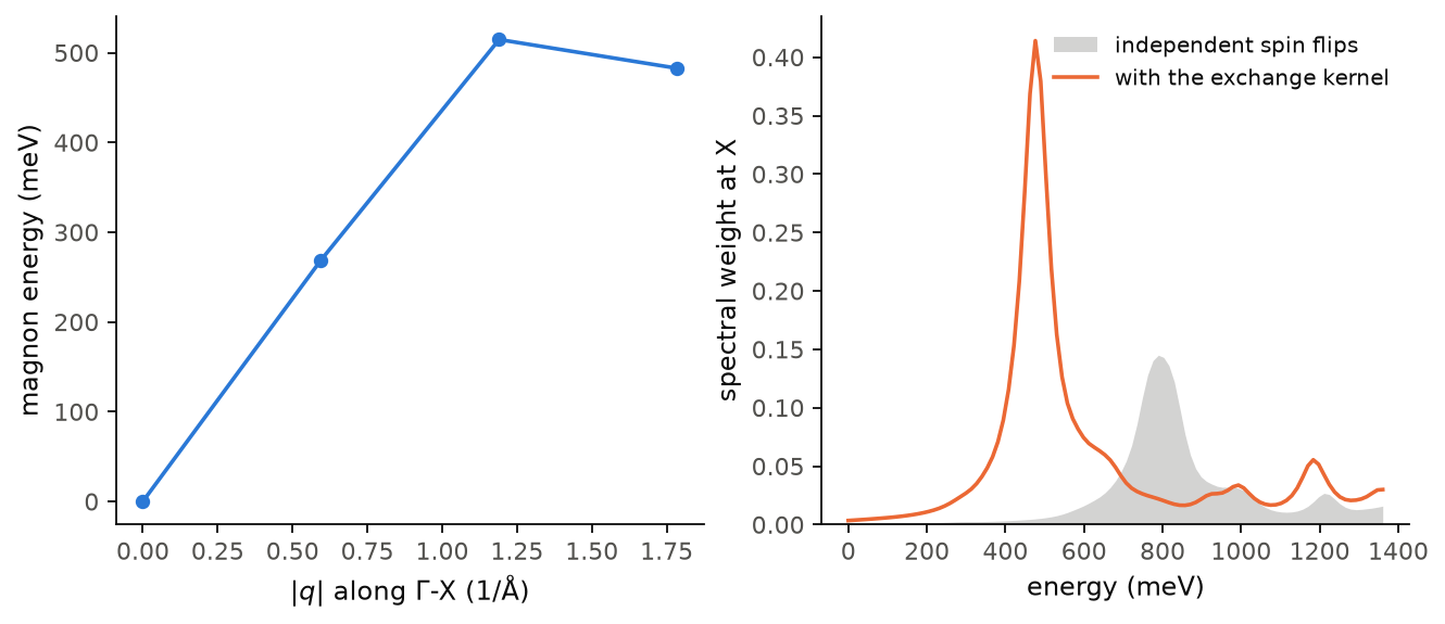
Here we follow the magnon of nickel from \(\Gamma\) to X, on a \(6\times6\times6\) mesh, so the wavevectors are \((0, s, s)\) with \(s = 0, 1/6, 1/3, 1/2\). On this mesh the moment is 0.624 \(\mu_B\) and the Goldstone miss is 2.2%. In the left panel we see that the magnon starts at zero energy at \(\Gamma\), as it must, and rises to 269 meV at 0.60 Å\(^{-1}\) and 515 meV at 1.19 Å\(^{-1}\), and then comes down a little to 483 meV at X. Four points are all that this mesh gives, so the curve between them is only a guide to the eye, and a finer mesh is what a real dispersion needs. The measured spin-wave stiffness of nickel, about 550 meV Å\(^2\), would give 195 meV at 0.60 Å\(^{-1}\), but the quadratic law holds only at smaller \(q\) than this mesh can reach. In the right panel we show the spectral function at X. The grey area is the Stoner continuum of independent spin flips, which peaks near 790 meV. With the exchange kernel, the weight moves into a sharp peak at 480 meV, below the continuum. This peak is the magnon, a collective mode in which no single electron flips its spin.

Code of this figure (docs/figures/magnons_dispersion/)

compute.py

"""The magnon of fcc nickel along Gamma-X, and the Stoner continuum."""
import numpy as np
from defuqumat import Calculator
from common import PSEUDO, save

# a q-point must be a difference of two k-points, so the mesh sets the q-points
text = open("ni.in").read().replace(" 4 4 4 0 0 0", " 6 6 6 0 0 0")
nickel = Calculator.from_text(text, pseudo_dir=PSEUDO)
s = np.arange(4) / 6                                # (0, s, s): Gamma to X
qpoints = [(0.0, x, x) for x in s]
frequencies = np.linspace(0.0, 0.1, 101)            # Ry
disp = nickel.get_magnon_dispersion(qpoints, frequencies, nbnd=24, ecut_response=40.0,
                                    broadening=3e-3, goldstone_correction=True)
for q, w, lam in zip(qpoints, disp.energies_mev, disp.enhancements):
    print(f"q = {q}   magnon {w:.0f} meV   enhancement {lam:.4f}", flush=True)

alat = float(nickel.system.cell.alat)
save(q=s * 2 * np.pi / alat * 2 / 0.529177,        # |q| in 1/Angstrom, (0, s, s) = (0, 2s, 0) 2pi/a
     magnon=disp.energies_mev, enhancement=disp.enhancements,
     goldstone=disp.goldstone, moment=nickel.get_scf().magnetization,
     energies=frequencies * 13605.693,
     spectral=np.array([c.spectral_function for c in disp.susceptibilities]),
     stoner=np.array([c.kohn_sham_spectral_function for c in disp.susceptibilities]))

plot.py

"""The magnon energy along Gamma-X, and the spectral function at the last q."""
import numpy as np
import style

d = np.load("data.npz")


def draw():
    fig, (a, b) = style.figure(2)
    a.plot(d["q"], d["magnon"], "o-")
    a.set_xlabel(r"$|q|$ along $\Gamma$-X (1/Å)")
    a.set_ylabel("magnon energy (meV)")
    i = len(d["q"]) - 1
    b.fill_between(d["energies"], d["stoner"][i], color=style.ink2(), alpha=0.25, lw=0,
                   label="independent spin flips")
    b.plot(d["energies"], d["spectral"][i], color=style.color(1),
           label="with the exchange kernel")
    b.set_xlabel("energy (meV)")
    b.set_ylabel("spectral weight at X")
    b.set_ylim(bottom=0.0)
    b.legend()
    return fig


style.main(draw)

Limits

Magnons need nspin = 2, because without a collinear magnetization there is no transverse channel and the kernel \(B_{xc}/m\) does not exist. A spinor run (noncolin = .true.) works when its moment points along \(z\) and there is no spin-orbit coupling. It gives the same numbers as the nspin = 2 run. A noncollinear texture gives an error, since it needs the full \(4\times4\) spin-density response. Spin-orbit coupling and an ultrasoft spinor run give an error.

Magnons need the full k-mesh, so a symmetry-reduced k-set gives an error and you run with nosym = .true. and noinv = .true.. The reason is that \(\chi_0^{+-}(\mathbf G,\mathbf G')\) is a matrix in two \(\mathbf G\) indices that we do not symmetrise, and the states at \(\mathbf k + \mathbf q\) must come from the same mesh. A \(\mathbf q\) that is not a difference of two k-points of the mesh gives an error. A negative ecut_response gives an error, while ecut_response = 0 keeps \(\mathbf G = 0\) alone.

A PAW dataset gives an error, because its exchange field has a part on the spheres that the kernel does not see, so the enhancement would be wrong. Ultrasoft datasets work, and we include their augmentation charge in every matrix element.

A spin spiral gives an error, because its two spinor components live on plane-wave spheres centred at \(\mathbf k\) plus and minus half the spiral wave vector, and the matrix elements we compute need one sphere. A Hubbard \(U\) works with the simplified functional. The response then has one more entry for each pair of orbitals of a correlated atom, and you pass nothing new. A Hubbard \(J\) (the full functional) and BETA give an error.

A uniform B_field works. The magnon at \(\mathbf q = 0\) then sits at the Zeeman energy \(2B\), not at zero, and .goldstone is read there. .larmor gives this energy. A constrained moment gives an error, because it changes the functional. A LOCAL_MAGNETIC_FIELDS card gives an error, because a field inside spheres has no single Zeeman energy. A potential-only meta-GGA gives an error, because it has no exchange-correlation energy, and the kernel comes from the energy staying the same under a global spin rotation. A run with nosource gives an error, because the kernel \(B_{xc}/m\) is a scalar only while \(B_{xc}\) is parallel to \(\mathbf m\), which is what the source-free projection breaks.

goldstone_correction=True with interacting=False gives an error, because the correction needs the interacting response at \(\mathbf q = 0\).

The notebook for this page is 38, magnons.