Spin-orbit coupling

In this page we switch on spin-orbit coupling. We see the gap it opens in a heavy element, and then we compute the orbital moment on each atom and of the whole cell.

Spinors and fully relativistic pseudopotentials

We start with the spinors. With noncolin = .true. a wavefunction is a spinor with two components, so there is one Hamiltonian on a space twice as large. lspinorb = .true. then adds the coupling of the spin to the orbital motion,

\[ H_{\rm SO} \propto \boldsymbol\sigma \cdot \mathbf L , \]

through a fully relativistic pseudopotential (a file with rel in its name). Such a file has two projectors for each \(l\), one for \(j = l - \tfrac12\) and one for \(j = l + \tfrac12\). A scalar-relativistic file has one, their average, and the difference of the two is the coupling. Spin-orbit coupling is what gives rise to the Rashba splitting that ARPES sees, the gap of a topological insulator, and the magnetic anisotropy of a magnet. Here we take bismuthene:

import numpy as np
from defuqumat import Calculator
from defuqumat.units import RY_TO_EV

calc = Calculator.from_file("docs/figures/spin-orbit_bismuthene/bi-soc.in",
                            pseudo_dir="tests/data/pseudo")
scf = calc.get_scf()
print(calc.system.nspin, calc.system.npol)
print(np.round(scf.eigenvalues[0, 24:34] * RY_TO_EV, 4))   # eV, first k-point

4 2
[-3.9727 -3.9727 -3.1025 -3.1025 -2.4528 -2.4528  0.3142  0.3142  0.9062
  0.9062]

A spinor run has nspin = 4 and npol = 2. Each band holds one electron, so a run has twice as many bands as without spinors. Bismuthene has inversion and time-reversal symmetry, and together they keep every level doubly degenerate, however strong the coupling is. This is Kramers' theorem, and we see it in the pairs above. The code does not impose it. You can also switch the coupling off inside the same fully relativistic file with soc_scale = 0, or scale it with a value between 0 and 1, which is useful to see which part of a result comes from the coupling.

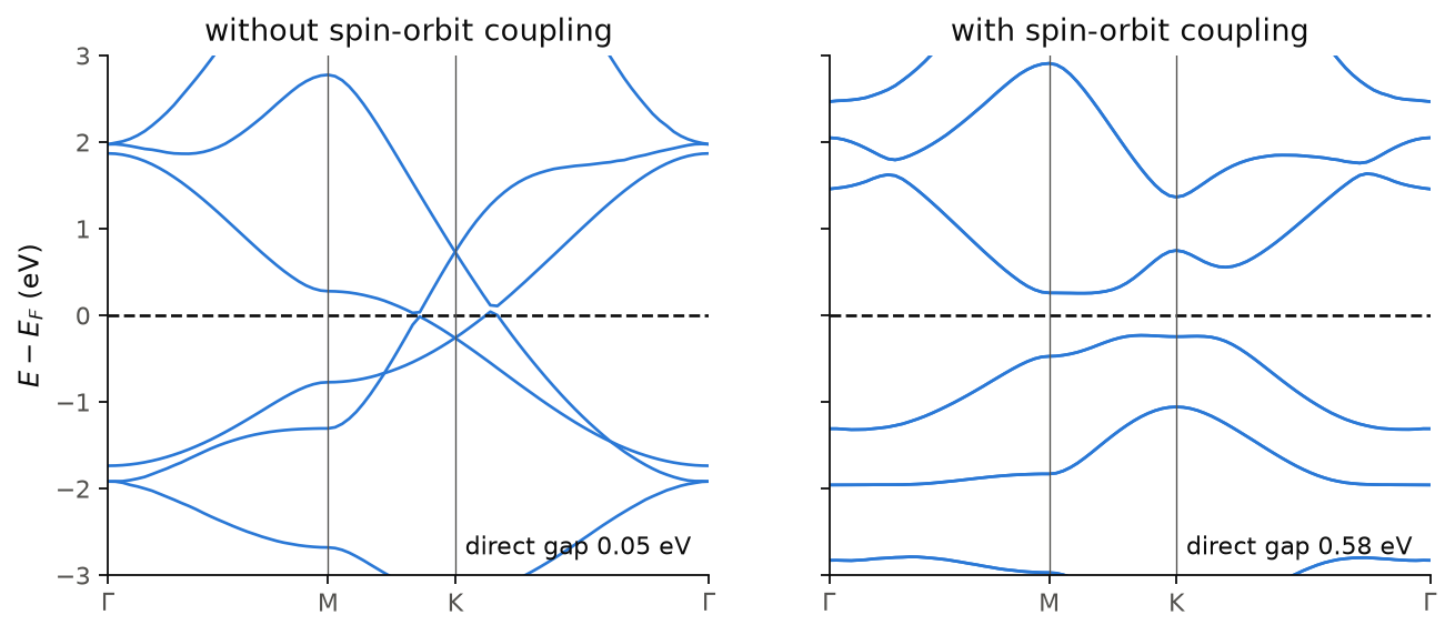
The figure shows bismuthene, a honeycomb layer of bismuth, at a small cutoff and on a \(6\times6\times1\) mesh. The two runs differ only in noncolin, lspinorb and the pseudopotential file. Without the coupling, two bands nearly touch between M and K, 0.05 eV apart. The valence and the conduction bands also overlap in energy, by 0.01 eV, so the layer is a semimetal. With the coupling a gap opens everywhere on the path. The smallest direct gap is 0.58 eV, and the indirect gap is 0.49 eV, from the top of the valence band near K to the bottom of the conduction band at M. This gap comes only from the coupling, and it makes bismuthene a quantum spin Hall insulator. We compute its \(Z_2\) invariant in the page about topology.

Code of this figure (docs/figures/spin-orbit_bismuthene/)

compute.py

"""The bands of bismuthene without and with spin-orbit coupling."""
import numpy as np
from defuqumat import Calculator
from defuqumat.system.kpoints import KPoints
from defuqumat.units import RY_TO_EV
from common import PSEUDO, save

corners = [[0.0, 0.0, 0.0], [0.5, 0.0, 0.0], [1 / 3, 1 / 3, 0.0], [0.0, 0.0, 0.0]]
counts = [30, 18, 36, 1]                      # Gamma - M - K - Gamma, crystal units
data = {}
for tag, nbnd, filled in (("nosoc", 20, 15), ("soc", 40, 30)):   # 30 electrons
    calc = Calculator.from_file(f"bi-{tag}.in", pseudo_dir=PSEUDO)
    scf = calc.get_scf()
    path = KPoints.band_path(corners, counts, calc.system.cell, crystal=True)
    bands = calc.get_bands(kpoints=path, nbnd=nbnd)
    e = bands.eigenvalues_ev - scf.fermi_energy * RY_TO_EV
    data[tag] = e
    data[tag + "_gap"] = (e[:, filled] - e[:, filled - 1]).min()   # smallest direct gap
    print(tag, "smallest direct gap %.4f eV" % data[tag + "_gap"], flush=True)

save(x=bands.path_length, ticks=bands.path_length[np.cumsum([0] + counts[:-1])], **data)

plot.py

"""Bismuthene: the bands without and with spin-orbit coupling."""
import numpy as np
import style

d = np.load("data.npz")


def draw():
    fig, axes = style.figure(2, sharey=True)
    for ax, tag, title in zip(axes, ("nosoc", "soc"),
                              ("without spin-orbit coupling", "with spin-orbit coupling")):
        ax.plot(d["x"], d[tag], color=style.color(0), lw=1.2)
        ax.axhline(0.0, **style.reference())
        for t in d["ticks"][1:-1]:
            ax.axvline(t, color=style.ink2(), lw=0.6)
        ax.set_xticks(d["ticks"], [r"$\Gamma$", "M", "K", r"$\Gamma$"])
        ax.set_xlim(d["x"][0], d["x"][-1])
        ax.set_ylim(-3.0, 3.0)
        ax.set_title(title)
        ax.text(0.97, 0.04, "direct gap %.2f eV" % d[tag + "_gap"],
                transform=ax.transAxes, ha="right")
    axes[0].set_ylabel(r"$E - E_F$ (eV)")
    return fig


style.main(draw)

The angular momenta on each atom

Let us now ask where a moment lives, and how much of it is orbital. We project the states on the atomic orbitals of each atom, as for the projected DOS, and we take the expectation values of \(\mathbf L\) and of \(\mathbf S = \boldsymbol\sigma/2\):

\[ \langle L_i\rangle = \sum_s \mathrm{Tr}_m \left(L_i\,\rho_{ss}\right), \qquad \langle S_i\rangle = \tfrac12 \sum_m \mathrm{Tr}_s\left(\sigma_i\,\rho_{mm}\right), \qquad \mathbf J = \mathbf L + \mathbf S . \]

XMCD measures the orbital and the spin moment of an element apart, with its sum rules. Here we take fcc nickel with spin-orbit coupling and the moment along \(z\):

nickel = Calculator.from_file("docs/figures/spin-orbit_bismuthene/ni-soc.in",
                              pseudo_dir="tests/data/pseudo")
print(nickel.get_angular_momenta().table())

Angular momenta on the ortho-atomic projectors (units of hbar)

  Ni1  L = (-0.00000,-0.00000, 0.03647)  S = (-0.00001,-0.00000, 0.31270)  J = (-0.00001,-0.00000, 0.34918)

  total L = (-0.00000,-0.00000, 0.03647)
  total S = (-0.00001,-0.00000, 0.31270)

The values are in units of \(\hbar\). We see that \(\langle L_z\rangle = 0.036\,\hbar\) is parallel to \(\langle S_z\rangle\), as Hund's third rule says for a shell that is more than half full. The ratio \(|L|/|S| = 0.117\) is close to the measured value of about 0.1. Without spin-orbit coupling \(\langle L\rangle\) is zero, because the crystal field quenches it. The result has .atoms, with .l, .s and .j for each atom, and .orbital and .spin as arrays with one row per atom.

The orbital magnetization of the cell

We now compute the orbital moment of the whole cell. The orbital moment of a crystal is not the sum of the moments on its atoms, because the currents of the Bloch states run through the whole crystal. So \(\int \mathbf r\times\mathbf j\) depends on where you cut the cell, as for the polarization. The quantity that is well defined is an integral over the Brillouin zone (the modern theory of the orbital magnetization):

\[ \mathbf M = \frac{e}{2\hbar c}\,\mathrm{Im} \sum_n \int \frac{d\mathbf k}{(2\pi)^3}\, \big\langle \partial_{\mathbf k} u_n \big| \times \big( H_{\mathbf k} + \varepsilon_{n\mathbf k} - 2\mu \big) \big| \partial_{\mathbf k} u_n \big\rangle . \]

It has a local and an itinerant part, and only their sum is measurable. It needs broken time reversal (a magnet) and spin-orbit coupling. Here we take one iodine atom in a box, \(5s^2 5p^5\), with one hole in the \(p\) shell:

iodine = Calculator.from_file("docs/figures/spin-orbit_bismuthene/iodine.in",
                              pseudo_dir="tests/data/pseudo")
orbm = iodine.get_orbital_magnetization(divisions=(3, 3, 3))
print(f"local      {orbm.lc[2]:.5f} mu_B")
print(f"itinerant  {orbm.ic[2]:.5f} mu_B")
print(f"total      {orbm.total[2]:.5f} mu_B")

local      -0.59864 mu_B
itinerant  -0.57580 mu_B
total      -1.17444 mu_B

The total is \(-1.17\,\mu_B\), about one Bohr magneton, as Hund's rules ask for a \(p\) shell with one hole and \(L = 1\). The sign is the charge of the electron. The local and the itinerant parts are nearly equal here, but only their sum is a physical quantity. orbm.lc, orbm.ic and orbm.total are vectors in \(\mu_B\) per cell, and divisions is the k-mesh of the derivative. The occupied states must be separated from the empty ones by a gap, which is why the input uses fixed occupations. This is the quantity pw.x computes with lorbm.

Limits

A spin spiral with spin-orbit coupling gives an error, because the coupling breaks the generalized Bloch theorem that the spiral rests on. At soc_scale = 0 a fully relativistic file is accepted.

For a fully relativistic ultrasoft or PAW dataset, the site angular momenta use the \(|l\,j\,m_j\rangle\) orbitals of projwfc.x. So the charge on each atom is the Löwdin charge of projwfc.x. In such a file the two \(j\) shells of one \(l\) have two radial functions. \(\langle L\rangle\) and \(\langle S\rangle\) treat them as one function. On cobalt with the coupling switched off, this gives \(|\langle L\rangle| = 1\times10^{-3}\,\hbar\), where the exact value is zero. With the coupling on, it changes \(\langle L\rangle\) by 1.7 per cent. A norm-conserving spin spiral works, and each spinor component is projected on the atomic orbitals of its own sphere. An ultrasoft or PAW spiral gives an error. A run with K_POINTS gamma works, and a k-set reduced by symmetry works.

The orbital magnetization gives an error for an ultrasoft or PAW dataset, as in pw.x. It gives an error without spinors (noncolin = .false.) and for nspin = 2, because there the orbital moment is zero. A spinor run without the coupling is accepted and gives zero. A metal gives an error, and so does any occupied manifold whose gap to the band above is smaller than gap_tol (1e-4 Ry by default) at some k-point. A spin spiral gives an error. A mesh with two divisions along a direction gives an error, because the two neighbours of a point are then the same k-point. One division is allowed and sets that derivative to zero, as for a slab. Without divisions, k-points that do not come from a uniform grid give an error.

A spinor run has no elastic constants and no electrostriction. get_forces(method="analytic") gives an error for a spinor run, while the default forces and the stress work.

The notebooks for this page are 08, spin-orbit coupling, 29, effective mass and angular momenta and 39, orbital magnetization.