Nonlinear optics

In this page we compute the response of a crystal at second and third order in the light field: the shift current, the second harmonic, the current under a strong laser pulse with its high harmonics, and the third harmonic. The second order is zero in any crystal with an inversion centre, so we take zincblende AlAs, which has none, and silicon, which has one and is the control.

The shift current

We start with the simplest second-order effect, a direct current under uniform light. A crystal without an inversion centre carries this current with no junction and no built-in field, which is the bulk photovoltaic effect. Its intrinsic part is the shift current: the electron excited by the photon is born at a different place than the hole it leaves, and this shift per absorbed photon is the current. The current is second order in the field,

\[ J^a = 2\,\sigma^{abc}(0;\omega,-\omega)\,E_b(\omega)\,E_c(-\omega), \qquad \sigma^{abc}(\omega) = -\frac{i\pi e^3}{4\hbar^2}\int[d\mathbf k] \sum_{nm} f_{nm}\big(r^b_{mn} r^{c;a}_{nm} + r^c_{mn} r^{b;a}_{nm}\big) \big[\delta(\omega_{mn}-\omega)+\delta(\omega_{nm}-\omega)\big], \]

where \(r^b_{mn}\) is the interband dipole and \(r^{c;a}_{nm}\) its generalized derivative in \(\mathbf k\), which measures how far the charge centre moves in the transition. So \(\sigma^{abc}\) is the absorption times a length. It is a polar tensor of rank 3, so it is zero in a crystal with an inversion centre, and it is zero below the gap, where no photon is absorbed. This current is what a photovoltaic measurement on a single crystal with no contacts in the light sees. We compute it with calc.get_shift_current():

from defuqumat import Calculator

alas = Calculator.from_file("docs/figures/nonlinear_shg/alas.in",
                            pseudo_dir="tests/data/pseudo")
sigma = alas.get_shift_current(nbnd=14, window=0.9, nw=180)

xyz = sigma.component(0, 1, 2)             # sigma^xyz in A/V^2
i = abs(xyz).argmax()
print(f"largest sigma_xyz: {xyz[i] * 1e6:.1f} uA/V^2 at {sigma.frequencies_ev[i]:.2f} eV")
print(f"truncation: {100 * sigma.truncation:.1f} per cent")

largest sigma_xyz: -33.8 uA/V^2 at 4.17 eV
truncation: 5.7 per cent

sigma.sigma is the whole tensor, with the shape (nw, 3, 3, 3) and in A/V\(^2\), and sigma.frequencies_ev is the photon energy. In zincblende the only components that are not zero are the six with three different labels, and they are all equal, so \(\sigma^{xyz}\) is the whole answer. We see that the largest current in magnitude, 33.8 \(\mu\)A/V\(^2\), comes at 4.17 eV, far above the smallest direct gap of this mesh, 2.42 eV, and below the gap there is no current at all, since no photon is absorbed. With 14 bands the truncation is 5.7 per cent, so the number is good to a few per cent and not better. Note that some papers write \(J = \sigma E E\) without the factor 2 and so report numbers twice as large for the same physics. You check the convention before you compare.

The keywords of get_shift_current and of get_shg below are:

• nbnd: the number of bands in the sums. It is required, and it is the convergence parameter of the whole quantity, because the sum over the intermediate state is exact only over a complete basis. .truncation is the change of the result when the top quarter of the bands is left out, so you read it before you trust a number.
• kpoints: a denser k-set to evaluate on. It can be the whole unshifted grid or its wedge. If you do not give it, the code uses the k-points of the SCF.
• window, nw, frequencies: the photon energies, as a window in Ry with nw points or as an explicit list in Ry.
• broadening: the width of the resonances, in Ry.
• scissor (get_shg only): a rigid shift of the empty bands in Ry, to correct the gap of the LDA or the GGA.

Second-harmonic generation

Let us now send light of frequency \(\omega\) into the crystal and ask how much comes back at \(2\omega\). This is second-harmonic generation, the effect that turns the 1064 nm light of a Nd:YAG laser into green light at 532 nm. The polarization at \(2\omega\) is

\[ P^a(2\omega) = \chi^{abc}(-2\omega;\omega,\omega)\,E_b(\omega)\,E_c(\omega), \qquad \chi^{abc} = \frac{1}{\Omega}\sum_{\mathbf k,mn} \left[\frac{c^{(1)}_{mn}}{\omega_{mn}-\omega+i\eta} + \frac{c^{(2)}_{mn}}{\omega_{mn}-2(\omega-i\eta)}\right], \]

where the coefficients \(c^{(1,2)}_{mn}\) are products of three interband dipoles, summed over an intermediate band. So there are two kinds of resonance, one when a single photon reaches a transition and one when two photons do. Like the shift current, \(\chi^{abc}\) is a polar tensor of rank 3 and it is zero with an inversion centre. In zincblende only one independent component is left, \(\chi^{xyz}\), and the five other components with three different labels are equal to it. The intensity of the second harmonic, measured in a doubling experiment, goes as \(|\chi|^2\). We compute it with calc.get_shg():

chi = alas.get_shg(nbnd=23, window=0.6, nw=240, broadening=0.010)

xyz = chi.component(0, 1, 2)               # chi^xyz in pm/V, complex
print(f"chi_xyz at {chi.frequencies_ev[0]:.2f} eV: {xyz[0].real:.1f} pm/V, "
      f"d_xyz = {chi.d_coefficient(0, 1, 2)[0].real:.1f} pm/V")
i = abs(xyz).argmax()
print(f"largest |chi_xyz|: {abs(xyz[i]):.1f} pm/V at {chi.frequencies_ev[i]:.2f} eV")
print(f"truncation: {chi.truncation:.1e} of the peak")

chi_xyz at 0.00 eV: -108.9 pm/V, d_xyz = -54.4 pm/V
largest |chi_xyz|: 657.1 pm/V at 2.66 eV
truncation: 9.7e-03 of the peak

chi.chi is the whole complex tensor in pm/V, with the shape (nw, 3, 3, 3), and chi.frequencies_ev is the energy of the photon that goes in, not of the one that comes out. Many papers quote \(d = \chi/2\) instead of \(\chi\), and chi.d_coefficient(a, b, c) gives it, so you compare \(d\) with \(d\). The three physical parts of the sum, the pure interband term, its modulation by the intraband motion and the modulation of the transition energy, are in chi.chi_ii, chi.eta_ii and chi.sigma_ii. This run uses the \(4\times4\times4\) mesh of the input, which is too coarse for this quantity: on the \(6\times6\times6\) mesh of the figure the static value is \(-78.5\) pm/V and the peak is at 2.15 eV. The band truncation, 1 per cent of the peak, is small next to this.

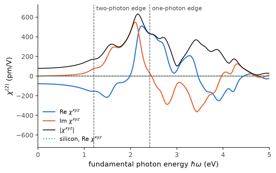
The figure shows \(\chi^{xyz}\) of AlAs on a denser \(6\times6\times6\) mesh, with 23 bands. The real part is \(-78.5\) pm/V at zero frequency. Below 1 eV the imaginary part is small, 6 pm/V at 0.5 eV, and this is only the tail of the broadening of 0.136 eV, so the crystal doubles light without absorbing it. The imaginary part grows fast from half the smallest direct gap of the SCF mesh, 1.21 eV, which is the two-photon edge. Here the photon that comes out, at \(2\hbar\omega\), reaches a real transition, while the light that goes in is not absorbed until the one-photon edge at 2.42 eV. The largest response, \(|\chi^{xyz}| = 632.9\) pm/V at 2.15 eV, sits between the two edges, so a crystal can be clear at \(\omega\) and opaque at \(2\omega\). These gaps are the gaps of the LDA, which is why scissor exists. The dotted line is silicon on the same mesh, and its largest component is \(5\times10^{-6}\) pm/V, which is zero within the numerical precision, as inversion demands. In AlAs the 21 components that zincblende forbids reach \(2\times10^{-8}\) of the peak, and nothing in the calculation imposes this pattern, since the sum runs over the whole mesh with no symmetry.

Code of this figure (docs/figures/nonlinear_shg/)

compute.py

"""The second-harmonic spectrum of AlAs, with silicon as the control."""
import numpy as np
from defuqumat import Calculator
from defuqumat.system.kpoints import KPoints
from defuqumat.units import RY_TO_EV
from common import PSEUDO, save

# AlAs: the ground state first (with empty bands, for the gap), then chi^(2) on a 6x6x6 mesh
alas = Calculator.from_file("alas.in", pseudo_dir=PSEUDO)
levels = np.asarray(alas.get_scf(nbnd=12).eigenvalues)
gap = (levels[:, 4] - levels[:, 3]).min() * RY_TO_EV          # the smallest direct gap
mesh = KPoints.automatic((6, 6, 6), (0, 0, 0), alas.system.cell)
chi = alas.get_shg(kpoints=mesh, nbnd=23, window=0.6, nw=240, broadening=0.010)

# silicon: the same calculation, where inversion forbids every component
silicon = Calculator.from_file("si.in", pseudo_dir=PSEUDO)
si_mesh = KPoints.automatic((6, 6, 6), (0, 0, 0), silicon.system.cell)
si_chi = silicon.get_shg(kpoints=si_mesh, nbnd=14, window=0.6, nw=240, broadening=0.010)

allowed = [(0, 1, 2), (0, 2, 1), (1, 0, 2), (1, 2, 0), (2, 0, 1), (2, 1, 0)]
forbidden = max(np.abs(chi.component(a, b, c)).max() for a in range(3) for b in range(3)
                for c in range(3) if (a, b, c) not in allowed)
save(ev=chi.frequencies_ev, xyz=chi.component(0, 1, 2), gap=gap,
     si_ev=si_chi.frequencies_ev, si_xyz=si_chi.component(0, 1, 2),
     si_peak=np.abs(si_chi.chi).max(), forbidden=forbidden,
     truncation=chi.truncation)

plot.py

"""The second-harmonic susceptibility of AlAs, and of silicon as the control."""
import numpy as np
import style

d = np.load("data.npz")


def draw():
    fig, ax = style.figure()
    xyz = d["xyz"]
    ax.plot(d["ev"], xyz.real, color=style.color(0), label=r"Re $\chi^{xyz}$")
    ax.plot(d["ev"], xyz.imag, color=style.color(1), label=r"Im $\chi^{xyz}$")
    ax.plot(d["ev"], np.abs(xyz), color=style.ink(), lw=1.2, label=r"$|\chi^{xyz}|$")
    ax.plot(d["si_ev"], d["si_xyz"].real, color=style.color(2), ls=":",
            label=r"silicon, Re $\chi^{xyz}$")
    style.zero_line(ax)
    top = 1.15 * np.abs(xyz).max()
    for edge, name in ((d["gap"] / 2, "two-photon edge"), (d["gap"], "one-photon edge")):
        ax.axvline(edge, color=style.ink2(), ls="--", lw=0.9)
        ax.text(edge + 0.05, 0.92 * top, name, color=style.ink2(), fontsize=9)
    ax.set_xlim(0.0, 5.0)
    ax.set_ylim(-top, top)
    ax.set_xlabel(r"fundamental photon energy $\hbar\omega$ (eV)")
    ax.set_ylabel(r"$\chi^{(2)}$ (pm/V)")
    ax.legend(loc="lower left")
    return fig


style.main(draw)

The current under a laser pulse

So far the field was weak and we expanded the current in powers of it. We now take a strong pulse and follow the electrons in time, with no expansion. The field enters as a shift of every crystal momentum by \(\boldsymbol\kappa(t) = \mathbf A(t)/c\), with \(\mathbf E = -\partial_t\boldsymbol\kappa\), so each occupied state evolves under the Bloch Hamiltonian at a displaced k-point,

\[ i\,\partial_t|u_{n\mathbf k}(t)\rangle = H\big(\mathbf k+\boldsymbol\kappa(t)\big)\,|u_{n\mathbf k}(t)\rangle, \qquad \mathbf J(t) = -\frac{1}{\Omega}\sum_{n\mathbf k} w_{n\mathbf k} \Big\langle u_{n\mathbf k}(t)\Big|\frac{\partial H}{\partial\mathbf k} \Big|_{\mathbf k+\boldsymbol\kappa(t)}\Big|u_{n\mathbf k}(t)\Big\rangle , \]

meaning that the current is the derivative of the band energy with respect to the shift, at fixed states. By default the potential stays at the one of the ground state, which is the independent-particle response. A pulse is an object that you build first, with its peak intensity in W/cm\(^2\), its photon energy in eV and its number of cycles. We compute the current with calc.get_realtime(pulse):

from defuqumat import Calculator
from defuqumat.realtime import Sin2

silicon = Calculator.from_file("docs/figures/nonlinear_hhg/si.in",
                               pseudo_dir="tests/data/pseudo")
pulse = Sin2.from_intensity(3e12, 1.55, 2, polarization=(1, 1, 1))  # W/cm^2, eV, cycles
run = silicon.get_realtime(pulse, dt=0.2, nbnd=8)

print(run.times.shape, run.current.shape)   # Hartree atomic units of time, J is (nt, 3)
print(f"duration {run.times_fs[-1]:.2f} fs, largest |J| {abs(run.current).max():.3e} a.u.")
print(f"work of the field {run.work:.4e} Ha, energy gained {run.energy_gained:.4e} Ha")
print(f"electrons left in the conduction bands: {run.excited:.3f} per cell")

(1105,) (1105, 3)
duration 5.34 fs, largest |J| 6.754e-04 a.u.
work of the field 3.4221e-02 Ha, energy gained 3.4220e-02 Ha
electrons left in the conduction bands: 0.215 per cell

The pulse is 800 nm light, 1.55 eV per photon, with a \(\sin^2\) envelope two cycles long and a peak intensity of \(3\times10^{12}\) W/cm\(^2\). run.current is the current density at each time of run.times, in Hartree atomic units, and run.efield and run.kappa are the field and the shift on the same times. Two numbers check the run. The work that the field does on the current, \(\Omega\int\mathbf J\cdot\mathbf E\,dt\), is the energy that the crystal gains, here to a few parts in \(10^5\). This check does not depend on the units, so it sees a step that does not conserve the norm or a current that is not the derivative of the Hamiltonian. And run.excited counts the electrons that the pulse leaves in the conduction bands, 0.215 per cell of the eight valence electrons after the pulse has passed, so this is real absorption and not only a polarization that follows the field.

The keywords of get_realtime, which the other real-time methods of this page take too, are:

• dt: the time step, in Hartree atomic units of time (24.19 as). The code gives an error for a step that is too long to be stable.
• grid: an unshifted Monkhorst-Pack mesh, for example (6, 6, 6). If you do not give it, the code uses the mesh of the input. The mesh is reduced with the symmetry operations of the crystal that leave the field unchanged.
• nbnd: the number of bands of the first diagonalization, before the occupied ones are kept.
• potential: "frozen" (the default) keeps the potential of the ground state. "hartree" updates the Hartree potential at every step, which gives the local fields, and "hxc" updates the Hartree and the exchange-correlation potentials, the adiabatic LDA for an LDA run.
• duration: the length of the run. If you do not give it, the run is the length of the pulse.

A kick, a step in \(\boldsymbol\kappa\) at \(t=0\), is a field that contains every frequency, so the current after it gives the linear response at all frequencies at once,

\[ \sigma_{ab}(\omega+i\eta) = -\frac{1}{\kappa_0}\int_0^\infty J_a(t)\,e^{i(\omega+i\eta)t}\,dt, \qquad \epsilon_{ab} = \delta_{ab} + \frac{4\pi i\,\sigma_{ab}}{\omega+i\eta} . \]

This is the dielectric function that ellipsometry measures. We compute it with calc.get_realtime_dielectric(), here with the frozen potential and with the Hartree and exchange-correlation potentials updated:

for potential in ("frozen", "hxc"):
    eps = silicon.get_realtime_dielectric(direction=(1, 0, 0), broadening=0.5,
                                          frequencies=[0.5, 2.0, 3.5], dt=0.2,
                                          subtract_static=True, potential=potential)
    print(potential, " ".join(f"{e:.2f}" for e in eps.epsilon[:, 0]))

frozen 23.73+0.71j 32.87+10.59j 8.82+39.77j
hxc 22.85+1.09j 31.57+10.13j 8.02+36.99j

Here broadening and the frequencies are in eV, and eps.epsilon[:, 0] is \(\epsilon_{xx}\) at the three energies. The local fields and the adiabatic LDA lower the response by roughly 4 per cent at 0.5 eV and by 7 per cent in the imaginary part at 3.5 eV, where the absorption is. Note that these values are those of the \(4\times4\times4\) mesh, which is far from converged for silicon, so \(\epsilon_{xx}\) reads 23.7 at 0.5 eV. On a coarse mesh the propagation also carries a false Drude term, a sum of the band curvature over the mesh that goes to zero only for a dense mesh and grows as \(1/\eta^2\) at low frequency. subtract_static=True removes the constant part of the current before the transform, which takes this term out, so you keep it on a coarse mesh and do not need it on a converged one.

High harmonics

Let us now drive the crystal hard. The pulse moves every electron a good part of the way across the Brillouin zone, where the band velocity is not linear in \(\mathbf k\), and it lifts some of them across the gap, so the current contains many multiples of the laser frequency. What a spectrometer behind the sample records is the power that this current radiates,

\[ S(\omega) = \big|\,\omega\,\mathbf J(\omega)\big|^2 . \]

This is high-harmonic generation, which in a solid is a probe of the band structure far from the band edges. We compute it with calc.get_hhg(pulse), which runs get_realtime and takes the spectrum of the current:

pulse = Sin2.from_intensity(3e12, 1.55, 8, polarization=(1, 1, 1))
hhg = silicon.get_hhg(pulse, dt=0.2, nbnd=8)
print(hhg.harmonics(7) / hhg.harmonic(1))   # orders 1 to 7, over the fundamental
print(hhg.cutoff(floor=1e-6))               # the last odd harmonic of the plateau

[1.00000000e+00 3.16619582e-02 2.12585978e+01 2.05726603e-02
 2.16976527e+00 1.81353720e-03 2.30727351e-01]
19

hhg.orders and hhg.total are the spectrum against the harmonic order, hhg.harmonic(n) is the peak at order \(n\), and hhg.realtime is the run of get_realtime behind it. get_hhg needs a pulse with a carrier frequency, so a kick goes to get_realtime_dielectric instead.

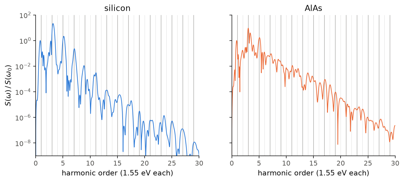
The figure shows the spectrum of silicon and of AlAs under the same pulse, \(3\times10^{12}\) W/cm\(^2\) at 1.55 eV, eight cycles long and polarized along \([111]\), on the \(4\times4\times4\) mesh of each input, divided by the peak at the fundamental. The dark lines mark the odd orders and the light ones the even orders. In silicon the peaks sit on the odd orders, and the third harmonic is 21 times the fundamental, the fifth 2.2 times and the seventh 0.23 times. The third harmonic is at 4.65 eV, above the direct gap, and \(S\) carries a factor \(\omega^2\), so a harmonic can be larger than the fundamental. Above the seventh order the peaks fall by a factor between 2.6 and 23 from one odd order to the next, and the last odd order above \(10^{-6}\) of the fundamental is the 19th. Inversion forbids the even orders, and what we read at them, \(3\times10^{-2}\) at the second order and \(2\times10^{-2}\) at the fourth, is the tail of the odd peaks next to them, since a pulse of eight cycles has a finite width in frequency. In AlAs, which has no inversion centre, the even orders are real: the second is 0.17 and the fourth 0.45 of the fundamental, twenty times silicon at the fourth order. The spectrum of AlAs also falls more slowly, and its last order above \(10^{-6}\) is the 25th. The pulse leaves 0.31 electrons per cell in the conduction bands of silicon and 0.42 in AlAs. These spectra use the mesh of the input and an independent-particle potential, so the height of each peak is not converged in \(\mathbf k\), while the selection of the orders by symmetry does not depend on the mesh.

Code of this figure (docs/figures/nonlinear_hhg/)

compute.py

"""High harmonics of silicon and AlAs under the same 800 nm pulse."""
from defuqumat import Calculator
from defuqumat.realtime import Sin2
from common import PSEUDO, save

# 3e12 W/cm^2, 1.55 eV photons, eight cycles, polarized along [111]
pulse = Sin2.from_intensity(3e12, 1.55, 8, polarization=(1, 1, 1))

out = {}
for name in ("si", "alas"):
    calc = Calculator.from_file(name + ".in", pseudo_dir=PSEUDO)
    hhg = calc.get_hhg(pulse, dt=0.2, nbnd=8)
    out[name + "_orders"] = hhg.orders
    out[name + "_total"] = hhg.total / hhg.harmonic(1)       # over the fundamental
    out[name + "_peaks"] = hhg.harmonics(30) / hhg.harmonic(1)
    out[name + "_cutoff"] = hhg.cutoff(floor=1e-6)
    out[name + "_excited"] = hhg.realtime.excited
save(**out)

plot.py

"""The high-harmonic spectra of silicon and AlAs under the same pulse."""
import numpy as np
import style

d = np.load("data.npz")


def draw():
    fig, axes = style.figure(2, sharey=True)
    for k, (ax, name, title) in enumerate(zip(axes, ("si", "alas"), ("silicon", "AlAs"))):
        for n in range(1, 31):
            ax.axvline(n, color=style.ink2(), lw=0.6 if n % 2 else 0.3,
                       alpha=0.6 if n % 2 else 0.3, zorder=0)
        ax.semilogy(d[name + "_orders"], d[name + "_total"], color=style.color(k), lw=1.0)
        ax.set_xlim(0, 30)
        ax.set_ylim(1e-9, 1e2)
        ax.set_xlabel("harmonic order (1.55 eV each)")
        ax.set_title(title)
    axes[0].set_ylabel(r"$S(\omega)\,/\,S(\omega_0)$")
    return fig


style.main(draw)

The orders of the current and the third harmonic

We now go back to a weak field and take each order of the current exactly. We scale the field, \(\boldsymbol\kappa(t) = \lambda\,\mathbf a(t)\), and expand \(\mathbf J = \sum_n \lambda^n \mathbf J^{(n)}\). The code takes each order as a derivative of the propagation with respect to \(\lambda\), so the orders come out separated, with no fit over several amplitudes. Under a field switched on slowly, \(\mathbf a(t) = e^{\eta t}\cos(\omega t)\,\hat{\mathbf e}\), the order \(n\) is

\[ \mathbf J^{(n)}(t) = e^{n\eta t}\sum_m \mathbf J_{(n,m)}\,e^{-im\omega t}, \]

so \(\mathbf J_{(n,m)}\) is the response of order \(n\) at the harmonic \(m\omega\), with a broadening \(\eta\) per photon. The third harmonic is \(\mathbf J_{(3,3)}\), the intensity-dependent refractive index (the optical Kerr effect) is \(\mathbf J_{(3,1)}\), and the second harmonic is \(\mathbf J_{(2,2)}\). With \(z = \omega + i\eta\), the third-order susceptibilities are

\[ \chi^{(3)}(-3\omega;\omega,\omega,\omega) = -\frac{8\,J_{(3,3)}}{3z^4}, \qquad \chi^{(3)}(-\omega;\omega,\omega,-\omega) = \frac{8\,J_{(3,1)}}{3(2z-\bar z)\,z^2\bar z}, \]

in atomic units. The third harmonic is what third-harmonic generation experiments measure, and \(\chi^{(3)}(-\omega;\omega,\omega,-\omega)\) gives the nonlinear refractive index \(n_2\) and the two-photon absorption. We compute the orders with calc.get_harmonic_orders() and \(\chi^{(3)}\) of a cubic crystal with calc.get_third_harmonic():

orders = silicon.get_harmonic_orders(frequency=1.55, broadening=0.3, order=3,
                                     grid=(2, 2, 2), eta_t=10)
for n, m in [(1, 1), (3, 1), (3, 3)]:
    print(f"J_({n},{m}) along x: {complex(orders.component(n, m, axis=0)):.3e}")

thg = silicon.get_third_harmonic(frequency=1.55, broadening=0.3, grid=(2, 2, 2), eta_t=10)
print(f"|chi_xxxx(3w)|      = {abs(thg.chi_xxxx_3w):.2e} m^2/V^2")
print(f"|chi_xxyy(3w)|      = {abs(thg.chi_xxyy_3w):.2e} m^2/V^2")
print(f"|chi_xxxx(w;w,w,-w)| = {abs(thg.chi_xxxx_w):.2e} m^2/V^2")

J_(1,1) along x: 2.647e-02+4.780e-03j
J_(3,1) along x: -1.829e+00-7.785e-01j
J_(3,3) along x: 1.976e-01-2.439e-01j
|chi_xxxx(3w)|      = 3.51e-18 m^2/V^2
|chi_xxyy(3w)|      = 1.74e-18 m^2/V^2
|chi_xxxx(w;w,w,-w)| = 1.96e-17 m^2/V^2

orders.component(n, m, axis) is \(J_{(n,m)}\) along one axis, in atomic units and per unit amplitude of the field to the power \(n\). Here frequency and broadening are in eV, and the field is switched on eta_t\(/\eta\) before \(t=0\), so a transient of about \(e^{-10}\), which is \(5\times10^{-5}\) of each order, is left from the start. get_third_harmonic runs a field along \([100]\) and one along \([110]\), which gives the two independent components of a cubic crystal, \(\chi_{xxxx}\) and \(\chi_{xxyy}\). In an isotropic medium \(\chi_{xxxx} = 3\chi_{xxyy}\) for the third harmonic, and here the ratio of the two magnitudes is 2.0 and not 3, so on this grid the response is not isotropic. These are numbers of a \(2\times2\times2\) grid, which is a check of the method and not a converged third harmonic, and this snippet took 730 s on one core, with its SCF, for this one frequency.

One propagation gives one frequency. For a spectrum, the code solves the same steady state directly at each frequency, with no time step. At order \(N\) and harmonic \(M\), each occupied state responds at the complex energy \(\epsilon_n + M\omega + iN\eta\), driven by the orders below through the derivatives of \(H(\mathbf k)\) along the field:

\[ \big(\epsilon_n + M\omega + iN\eta - H_0\big)\,c^{(N)}_M = \sum_{p=1}^{N}\frac{1}{p!\,2^p}\sum_{s=0}^{p}\binom{p}{s}\,h_p\, c^{(N-p)}_{M-(2s-p)}, \qquad h_p = \frac{\partial^p H(\mathbf k + x\hat{\mathbf e})}{\partial x^p}\Big|_{x=0} . \]

No sum over empty bands appears, so there is no band count to converge. We compute the spectrum with calc.get_nonlinear_spectrum(frequencies), here the second harmonic of AlAs and the third harmonic of silicon:

alas = Calculator.from_file("docs/figures/nonlinear_hhg/alas.in",
                            pseudo_dir="tests/data/pseudo")
spec = alas.get_nonlinear_spectrum([0.3, 1.2, 2.1], broadening=0.1,
                                   direction=(0, 1, 1), order=2)
for w, chi in zip(spec.frequencies, spec.chi2(axis=0)):   # chi_xyz, pm/V
    print(f"{w:.1f} eV  chi_xyz = {chi.real:7.1f} {chi.imag:+7.1f}i pm/V")

third = silicon.get_nonlinear_spectrum([1.0, 1.55, 2.0], broadening=0.2,
                                       direction=(1, 0, 0))
chi_3w, chi_w = third.chi3(axis=0)                 # m^2/V^2
for w, a, b in zip(third.frequencies, chi_3w, chi_w):
    print(f"{w:.2f} eV  |chi(3w)| = {abs(a):.2e}  |chi(w;w,w,-w)| = {abs(b):.2e} m^2/V^2")

0.3 eV  chi_xyz =    94.7    +2.7i pm/V
1.2 eV  chi_xyz =   214.5   +49.5i pm/V
2.1 eV  chi_xyz =  -510.5  +476.2i pm/V
1.00 eV  |chi(3w)| = 1.38e-17  |chi(w;w,w,-w)| = 2.40e-17 m^2/V^2
1.55 eV  |chi(3w)| = 1.69e-18  |chi(w;w,w,-w)| = 8.28e-18 m^2/V^2
2.00 eV  |chi(3w)| = 3.73e-19  |chi(w;w,w,-w)| = 6.70e-18 m^2/V^2

A field along \([011]\) gives \(\chi^{xyz}\) directly in the \(x\) component of the current, so spec.chi2(axis=0) is the one component of zincblende, with no factor. Along \([100]\) the same run gives nothing at \(2\omega\), because an operation of the crystal, the \(S_4\) about \(x\), reverses that field, and the second-order current does not change sign with the field, so its \(x\) component is zero. spec.component(n, m) is \(\mathbf J_{(n,m)}\) at every frequency, spec.chi3(axis) gives the two third-order susceptibilities, and with order=1 and potential="hxc", spec.epsilon(axis) is the dielectric function with local fields.

Note that this AlAs input is the 10 Ry one of the high-harmonic figure, so its numbers are not those of get_shg above at 30 Ry. There is also a convention to know: the steady state takes the response at \(\omega + i\eta\) and the electron charge \(-1\), while the sum over states of get_shg takes \(\omega - i\eta\) and no charge, so on the same crystal one is minus the complex conjugate of the other. This is why the static value is positive here and negative in get_shg.

The third harmonic of silicon falls by a factor of 37 from 1.0 to 2.0 eV, while the intensity-dependent part falls by a factor of 3.6. These are numbers of the \(4\times4\times4\) mesh of the input and not of silicon. The coupling to the field as a shift of crystal momentum leaves a term in each order that goes to zero only as the mesh converges, and at third order this term is as large as the answer on a coarse mesh, so a third harmonic of silicon needs a much denser grid. Each frequency costs nine linear solves per band and k-point, where the propagation needs a whole run, so the dense mesh is a job for get_nonlinear_spectrum, and get_harmonic_orders is its check at one frequency.

Limits

The shift current gives an error for an ultrasoft or PAW dataset, because one term, the second derivative of the projectors in \(\mathbf k\), is not implemented. It also gives an error for a spin spiral, DFT+U and a metal, where the partly filled bands give transitions of zero energy and every denominator of the sum diverges. A spinor run works, and so does a collinear spin-polarized run (nspin = 2), where the two channels add. With nspin = 2 it gives an error when tot_magnetization makes a channel stop inside a degenerate level, because the result then depends on an arbitrary choice inside the level.

Second-harmonic generation gives an error for a spin spiral, a metal and DFT+U. It works for a spinor run, for a collinear spin-polarized run (nspin = 2), where the two channels add, and for ultrasoft and PAW datasets. The static \(\chi^{(2)}\) and the electro-optic tensor of the Raman page still give an error, because that route needs a term which this sum over states does not use.

For both tensors a symmetry-reduced k-set is averaged over the group it was cut with, so the tensor is the same as on the whole mesh. A magnetic run, and a shifted mesh, still give an error. Then you pass the whole unshifted mesh as kpoints. The band count is not converged for you, so read .truncation. The code warns when nbnd cuts a degenerate level (band_cut_gap below \(10^{-8}\) Ry), because then the result depends on an arbitrary choice inside the level. For AlAs, 22 bands do that and 23 do not. The code also warns when a nosym run has an FFT grid that does not respect the fractional translations, which leaves a small false signal in a crystal where the tensor is zero, so for the SCF you keep the symmetry and pass the whole mesh as kpoints, as we do for silicon.

The real-time methods give an error for DFT+U, a spin spiral, a static electric field (tefield or lelfield), and a symmetry-reduced k-set passed as kpoints (you pass grid= instead, which builds the right reduction for the field). A ground state under a magnetic field or with a constrained moment works. The run uses the field that the SCF ended with, not the field in the input. With potential='hartree' or 'hxc', a penalty constraint (for example constrained_magnetization = 'atomic') gives an error. With potential='frozen' it works.

A shifted mesh works. It is not closed under the point group, so the code keeps only the operations that map the mesh onto itself. For silicon on 4 4 4 1 1 1 with a field along [100], that is two of eight, and 40 of 64 points. The result is the same as little_group=False to 1e-8. Note that a shifted mesh on a cubic cell is not cubic, so it gives a small current across the field that the crystal does not have. For a cubic cell, use an unshifted mesh. They also give an error when occupations = 'fixed' cuts a degenerate level, because the current then depends on an arbitrary choice inside the level, and for a time step that is too long to be stable.

A K_POINTS gamma ground state works. The states are solved again on the whole sphere, so the run costs twice the plane waves of the SCF.

A magnet, a spinor run with spin-orbit coupling, and ultrasoft and PAW datasets work in real time. With an ultrasoft or PAW dataset, the potential updated in time ("hartree" or "hxc") gives an error. A kick after the start of the run works, but it must land on a point of the time grid, so its time must be the start plus a whole number of steps dt. With the potential updated, a meta-GGA with "hxc" and a checkpoint give an error. A metal runs with the occupations of the ground state held fixed, and its intraband response converges slowly in \(\mathbf k\).

get_nonlinear_spectrum gives an error (HierarchyError, with its residual) when a solve or the outer solve does not converge, since an unconverged first order is amplified by \(1/(2\eta)\) in the second. It also gives an error for the potential updated in time above first order (the real-time route has it, one frequency per run), for a meta-GGA with "hxc", because its exchange-correlation kernel is not implemented, for an order above three, and for an nbnd that leaves no conduction band below the top four. A norm-conserving run with ecutrho above 4 ecutwfc works with the potential updated.

The notebooks for this page are 32, the shift current, 33, second-harmonic generation, 50, high harmonics and 51, nonlinear spectra.