STM images and tunnelling

In this page we compute what a scanning-tunnelling microscope sees. We start with the image of a surface at one bias, then we compute the spectrum \(\mathrm dI/\mathrm dV\) at one place, and finally we follow the electron through a two-dimensional material into a substrate below it, first in real space and then in momentum space.

The STM image

What does a scanning-tunnelling microscope see? In the picture of Tersoff and Hamann the tip is a point with no structure of its own, an s-wave tip, and the current it draws at \(\mathbf r\) is proportional to the local density of states of the sample at the tip:

\[ \rho_{\rm STM}(\mathbf r) = \sum_{n\mathbf k} w_{\mathbf k}\, \tilde\delta(E - \varepsilon_{n\mathbf k})\, |\psi_{n\mathbf k}(\mathbf r)|^2 , \]

with \(\tilde\delta\) a smeared delta function at the energy \(E\) of the tip, the Fermi level at zero bias. This is the density built from the states at one energy only, and not from all the occupied states, so an STM image is not a picture of the atoms and not a picture of the charge. It is a picture of the states near the Fermi level, seen in the vacuum where the tip is. The integral of \(\rho_{\rm STM}\) over the cell is the density of states \(D(E)\). A microscope records it in constant-height mode as a current and in constant-current mode as a height.

Here we take AB-stacked bilayer graphene, which is the top of a graphite crystal. Half of the atoms of the top layer, which we call A, sit on an atom of the layer below, and the other half, B, sit on the centre of a hexagon of the layer below. We compute the image with calc.get_stm():

from defuqumat import Calculator

graphite = Calculator.from_file("docs/figures/stm_graphite/graphite.in",
                                pseudo_dir="tests/data/pseudo")
image = graphite.get_stm(height=0.85, shape=(60, 60))

a, b, hollow = image.values[0, 0], image.values[40, 20], image.values[20, 40]
print(f"A {a:.3e}   B {b:.3e}   hexagon centre {hollow:.3e}   (1/(bohr^3 Ry))")
print(f"B/A = {b / a:.2f}")
print(f"integral over the cell {image.integral:.4f} states/Ry")

A 5.883e-04   B 9.649e-04   hexagon centre 2.408e-07   (1/(bohr^3 Ry))
B/A = 1.64
integral over the cell 2.4834 states/Ry

The two atoms of the top layer are both carbon and carry the same charge, and yet at the Fermi level B is 1.64 times brighter than A. You can think of it this way: A is bound to the atom below it, which pushes the states of A away from the Fermi level, so the states at the Fermi level sit on B. Above the centre of the hexagon the tip sees \(2.4\times10^{-7}\), more than three orders of magnitude less. So the brightest spot of each cell is on B, and A is 0.61 of it. This asymmetry between the two atoms is the origin of the triangular images of graphite, where only half of the atoms appear.

The integral of the image, 2.4834 states/Ry, is \(D(E_F)\) of the cell, here on the \(12\times12\times1\) k-mesh of the SCF with a Gaussian of 0.02 Ry. Bilayer graphene has very few states at the Fermi level, all near K, so this number depends strongly on the k-mesh, and in the next section the same width on a \(24\times24\times1\) mesh gives 0.6450 states/Ry. So this value is not converged. The ratio between B and A is the result that does not move: it is 1.62 on the finer mesh.

The keywords of get_stm are:

• height: the tip plane, as a crystal coordinate along the third lattice vector. Here 0.85 of \(c = 20\) bohr is 3.5 bohr above the top layer.
• plane: any other plane, given by three of its corners in crystal coordinates, the origin and the ends of the two edges. Use it for a cut that is not parallel to the surface, as the right panel of the figure below does.
• shape: the number of points on the plane. The value at each point is the exact plane-wave sum there, and not an interpolation.
• bias: the sample bias in Ry. If you do not give it, the tip sees a smeared delta at the Fermi level. With a bias, it sees all the states between \(E_F\) and \(E_F + V\), so a negative bias images the filled states and a positive bias the empty states.
• width, smearing: the width of the delta, in Ry, and its shape. If you do not give them, the code uses degauss of the run and a Gaussian.
• grid, nbnd: compute the bands again on a denser k-mesh, at fixed density, before building the image. A delta at the Fermi level needs more k-points than the SCF.
• mode: "constant-height", or "constant-current" with a set-point current and a scan range heights in bohr. In the second mode image.heights_bohr is the height of the tip at each point, which is the topograph a microscope records.
• spin, polarization: a magnetic tip, with its moment along a direction (nx, ny, nz), or "up" and "down" for a collinear run. The tip then sees \(\tfrac12[\rho + P\,\hat{\mathbf n}\cdot\mathbf m]\), so the image of a noncollinear magnet depends on where the tip points.

image.values is the image on the plane, image.coordinates the cartesian coordinates of its points in bohr, image.extent() the frame for imshow, and image.density the same quantity on the whole FFT grid of the cell.

Let us now open a window with the bias. With a bias, the values are a number of electrons per bohr\(^3\), and not a density of states:

for bias in (-0.15, 0.15):
    window = graphite.get_stm(height=0.85, shape=(60, 60), bias=bias)
    a, b = window.values[0, 0], window.values[40, 20]
    print(f"bias {bias:+.2f} Ry   A {a:.3e}   B {b:.3e}   B/A = {b / a:.2f}")

bias -0.15 Ry   A 1.909e-04   B 2.042e-04   B/A = 1.07
bias +0.15 Ry   A 2.793e-04   B 2.667e-04   B/A = 0.95

With a window of 0.15 Ry, about 2 eV, the contrast almost disappears: B/A is 1.07 for the filled states and 0.95 for the empty states. The window now collects states from a large part of the \(\pi\) bands, which sit on both atoms, and only the few states very near the Fermi level tell A and B apart. So the triangular image of graphite is a low-bias image.

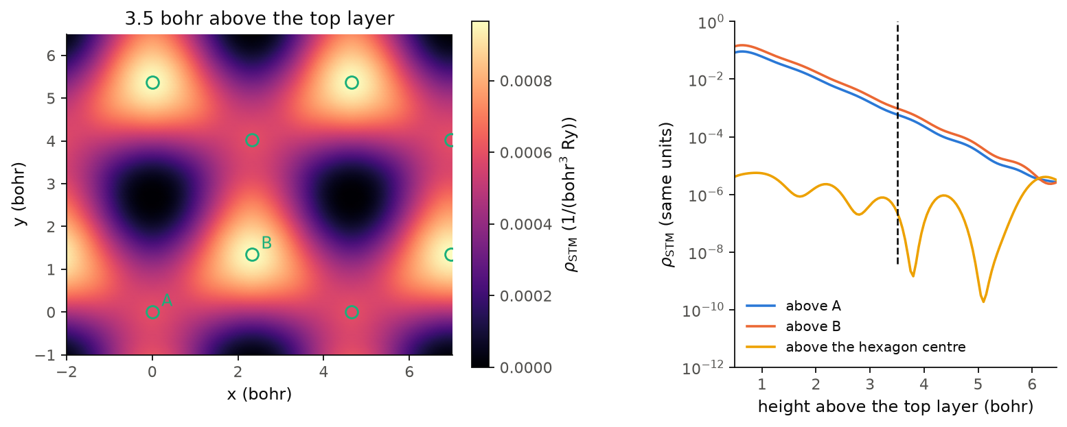
On the left we see the image at 3.5 bohr, repeated over a few cells. The bright spots are on B, A is dimmer but still bright, and only the centres of the hexagons are dark. On the right we follow the tunnelling density from the top layer up to the middle of the vacuum, 6.5 bohr. Above A and above B it falls by a factor of 10 every 1.16 bohr, and B stays brighter than A up to 6 bohr, so the contrast does not depend on the height of the tip. Above the centre of the hexagon the density stays below \(10^{-5}\) at every height. You can think of it this way: the states at the Fermi level are the states near K, and by the threefold symmetry the states of the top layer are zero on the axis through the centre of its hexagon. The small value left there comes from the atom of the lower layer that sits on this axis, 7.0 bohr further from the tip. At 6.5 bohr the three curves meet, near \(3\times10^{-6}\), because there the tip is as far from this surface as from the next copy of the slab, so the image has no contrast left.

The image here is at constant height. A microscope usually records the constant current mode, mode="constant-current", which needs the tip to reach the set-point everywhere, also above the dark centres of the hexagons. With 13 bohr of vacuum, as here, we stay with the constant-height image, which carries the same contrast, and for a topograph you need a cell with more vacuum.

Code of this figure (docs/figures/stm_graphite/)

compute.py

"""A constant-height STM image of graphite, and its decay into the vacuum."""
import numpy as np
from defuqumat import Calculator
from common import PSEUDO, save

calc = Calculator.from_file("graphite.in", pseudo_dir=PSEUDO)

# the tip plane at 0.85 of c, which is 3.5 bohr above the top layer (0.675)
image = calc.get_stm(height=0.85, shape=(60, 60))

# a vertical cut from the top layer (0.675) to the middle of the vacuum (1.0),
# through the atom A (0, 0), the hexagon centre (1/3, 2/3) and the atom B (2/3, 1/3);
# the plane is given by three corners in crystal coordinates
cut = calc.get_stm(plane=((0, 0, 0.675), (1, -1, 0.675), (0, 0, 1.0)), shape=(3, 130))
c = float(np.asarray(calc.system.cell.at)[2, 2])

save(xy=image.coordinates, image=image.values, integral=image.integral,
     z=np.arange(130) / 130 * 0.325 * c, decay=cut.values)

plot.py

"""The STM image of graphite at constant height, and the decay into the vacuum."""
import numpy as np
import style

d = np.load("data.npz")
xy = d["xy"]
n = xy.shape[0]
a1, a2 = n * (xy[1, 0] - xy[0, 0]), n * (xy[0, 1] - xy[0, 0])
f = np.arange(n + 1) / n                      # one cell, both edges included
x = f[:, None] * a1[0] + f[None, :] * a2[0]
y = f[:, None] * a1[1] + f[None, :] * a2[1]
image = np.pad(d["image"], ((0, 1), (0, 1)), mode="wrap")
atoms = {"A": (0, 0), "B": (2 / 3, 1 / 3)}


def draw():
    fig, (a, b) = style.figure(2, layout="constrained",
                              gridspec_kw={"width_ratios": [1.2, 1], "wspace": 0.15})
    for i in range(-1, 3):
        for j in range(-1, 3):
            shift = i * a1 + j * a2
            m = a.pcolormesh(x + shift[0], y + shift[1], image, shading="gouraud",
                             cmap=style.CMAP, vmin=0.0, vmax=image.max())
    for name, (f1, f2) in atoms.items():
        for i in range(-1, 3):
            for j in range(-1, 3):
                p = (f1 + i) * a1 + (f2 + j) * a2
                a.plot(*p, "o", mfc="none", mec=style.color(2), ms=8, mew=1.3)
        a.annotate(name, f1 * a1 + f2 * a2, color=style.color(2), xytext=(6, 4),
                   textcoords="offset points", fontsize=11)
    a.set_xlim(-2.0, 7.0)
    a.set_ylim(-1.0, 6.5)
    a.set_aspect("equal")
    a.set_xlabel("x (bohr)")
    a.set_ylabel("y (bohr)")
    a.set_title("3.5 bohr above the top layer")
    style.colorbar(fig, m, a, r"$\rho_{\rm STM}$ (1/(bohr$^3$ Ry))")

    for k, name, c in [(0, "above A", 0), (2, "above B", 1), (1, "above the hexagon centre", 3)]:
        b.semilogy(d["z"], d["decay"][k], color=style.color(c), label=name)
    b.axvline(3.5, ymin=0.3, **style.reference())       # the plane of the image
    b.set_xlim(0.5, d["z"][-1])
    b.set_ylim(1.0e-12, 1.0)
    b.set_xlabel("height above the top layer (bohr)")
    b.set_ylabel(r"$\rho_{\rm STM}$ (same units)")
    b.legend(loc="lower left")
    return fig


style.main(draw)

The tunnelling spectrum

An image is one energy at many places. Let us now take the other cut of the same function, one place at many energies, which is what a microscope measures when it holds the tip still and sweeps the bias:

\[ \frac{\mathrm dI}{\mathrm dV}(\mathbf r, V) \;\propto\; \rho(\mathbf r, E_F + eV) = \sum_{n\mathbf k} w_{\mathbf k}\, \tilde\delta(E_F + eV - \varepsilon_{n\mathbf k})\, |\psi_{n\mathbf k}(\mathbf r)|^2 . \]

This is scanning tunnelling spectroscopy (STS). It shows a gap, a band edge or a state inside a gap, which an image at one energy cannot show. The wavefunctions do not depend on the energy, so the code samples them at the tip once, and each energy after that costs almost nothing. We compute it with calc.get_sts():

import numpy as np

fermi = graphite.get_scf().fermi_energy
tips = [[0, 0, 0.85], [2 / 3, 1 / 3, 0.85]]         # above A and above B
sts = graphite.get_sts(energies=fermi + np.linspace(-0.3, 0.3, 121), tip=tips,
                       width=0.02, grid=(24, 24, 1), nbnd=16)

zero = np.argmin(np.abs(sts.bias_axis))
print(sts.values.shape)                              # (energies, tips)
print(f"dI/dV at V = 0:  A {sts.values[zero, 0]:.3e}   B {sts.values[zero, 1]:.3e}")
print(f"D(E_F) = {sts.integral[zero]:.4f} states/Ry per cell")

(121, 2)
dI/dV at V = 0:  A 1.538e-04   B 2.497e-04
D(E_F) = 0.6450 states/Ry per cell

At zero bias the tip above B sees 1.62 times more than the tip above A, the same contrast as in the image. Here the code computes the bands again on the full \(24\times24\times1\) mesh, 576 k-points, so \(D(E_F)\) is 0.6450 states/Ry per cell, against 2.4834 on the k-mesh of the SCF.

The keywords of get_sts are:

• energies: the energies of the tip, in Ry. There is no default, since the energy axis is the measurement.
• tip: the tip positions in crystal coordinates, one row each. One point gives a spectrum and a row of points a line cut. With height instead, the code gives a map at every energy.
• grid, nbnd: the k-mesh and the bands. A spectrum needs the full k-mesh, without symmetry, and grid builds it.
• width, smearing, spin, polarization: as for get_stm.

sts.values has the shape (energies, tips), sts.bias_axis is the bias in Ry measured from the Fermi level, sts.integral is \(D(E)\) per cell at each energy, and sts.current is \(I(V)\), the integral of the spectrum from \(V = 0\), negative for the filled states as in an experiment.

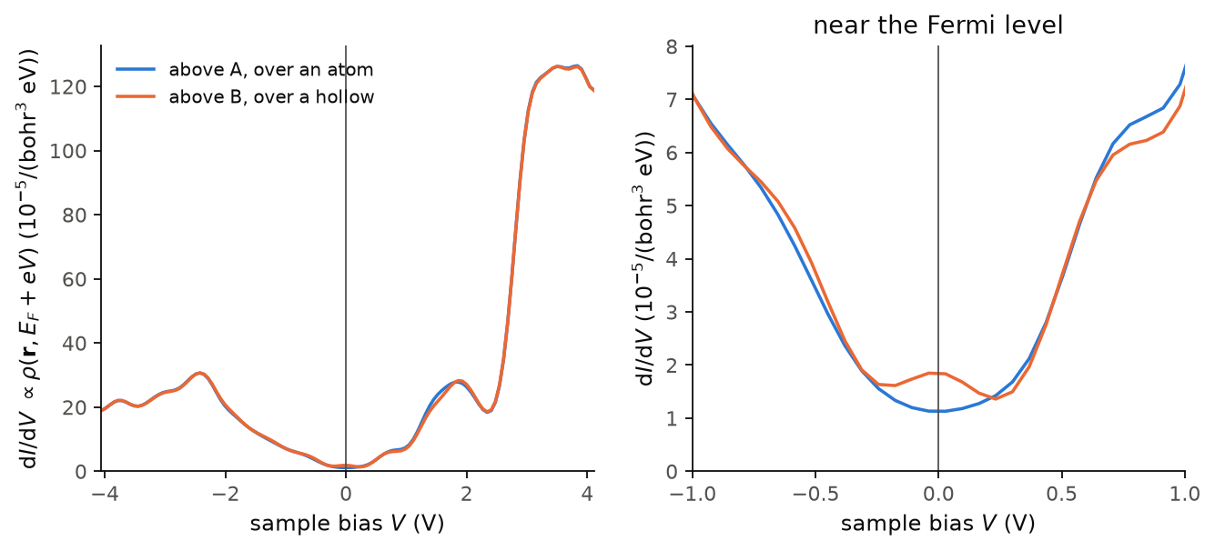
On the left we see the whole range, \(\pm 4\) V. The two curves are almost the same away from the Fermi level. The peak at \(-2.42\) V is the saddle point of the filled \(\pi\) band at M, a van Hove singularity, and the peak at \(+1.86\) V is its partner in the empty \(\pi^*\) band. Above about 2.7 V the signal grows by a factor of 4.5. These are states with much weight in the vacuum, and we did not converge them against the size of the vacuum, so this part of the curve depends on the cell. On the right we see the zoom near the Fermi level. Above A the spectrum has a minimum at \(V = 0\), which is the semimetal. Above B there is a small peak at \(V = 0\) instead, from the flat low-energy states of the bilayer, which sit on B. Only near zero bias A and B differ, with B up to 1.63 times A between \(-0.1\) and \(+0.1\) V. The width of the delta is 0.02 Ry, 0.27 eV, and the curve is smooth only because of this width. A sharper spectrum needs a denser k-mesh together with a smaller width.

Code of this figure (docs/figures/stm_spectrum/)

compute.py

"""Tunnelling spectra above the two kinds of surface atom of graphite."""
import numpy as np
from defuqumat import Calculator
from defuqumat.units import RY_TO_EV
from common import PSEUDO, save

calc = Calculator.from_file("graphite.in", pseudo_dir=PSEUDO)
fermi = calc.get_scf().fermi_energy

# the tip 3.5 bohr above the atom A (0, 0) and above the atom B (2/3, 1/3)
tips = [[0, 0, 0.85], [2 / 3, 1 / 3, 0.85]]
sts = calc.get_sts(energies=fermi + np.linspace(-0.3, 0.3, 121), tip=tips,
                   width=0.02, grid=(24, 24, 1), nbnd=16)

save(bias=sts.bias_axis * RY_TO_EV, didv=sts.values / RY_TO_EV,
     dos=sts.integral / RY_TO_EV)

plot.py

"""dI/dV above the two surface atoms of graphite, and a zoom near zero bias."""
import numpy as np
import style

d = np.load("data.npz")


def draw():
    fig, axes = style.figure(2)
    didv = d["didv"] * 1.0e5                       # in units of 1e-5/(bohr^3 eV)
    for ax, (lo, hi) in zip(axes, [(d["bias"][0], d["bias"][-1]), (-1.0, 1.0)]):
        ax.plot(d["bias"], didv[:, 0], color=style.color(0), label="above A, over an atom")
        ax.plot(d["bias"], didv[:, 1], color=style.color(1), label="above B, over a hollow")
        style.zero_line(ax, vertical=True)
        ax.set_xlim(lo, hi)
        ax.set_xlabel("sample bias $V$ (V)")
    near = np.abs(d["bias"]) <= 1.0
    axes[1].set_ylim(0.0, 1.1 * didv[near].max())
    axes[0].set_ylim(bottom=0.0)
    axes[0].set_ylabel(r"d$I$/d$V$ $\propto \rho(\mathbf{r}, E_F + eV)$ ($10^{-5}$/(bohr$^3$ eV))")
    axes[1].set_ylabel(r"d$I$/d$V$ ($10^{-5}$/(bohr$^3$ eV))")
    axes[0].legend(loc="upper left")
    axes[1].set_xticks([-1.0, -0.5, 0.0, 0.5, 1.0])
    axes[1].set_title("near the Fermi level")
    return fig


style.main(draw)

Vertical transport through a two-dimensional material

So far the tip only looks at the surface. We now ask a different question, what goes through. An electron enters at a point \(\mathbf r\) above a two-dimensional material and leaves into a substrate below it, an infinite flat plane. The current is then set by the amplitude to go from the tip to the plane, which is the nonlocal Green's function \(G(\mathbf r, \mathbf r')\), and not by the density of states at the tip:

\[ T(\mathbf r; E) = \int_{\rm plane} \bigl|G(\mathbf r, \mathbf r'; E)\bigr|^2\, d^2 r' , \qquad G(\mathbf r, \mathbf r'; E) = \sum_{n\mathbf k} \frac{\psi_{n\mathbf k}(\mathbf r)\,\psi^{*}_{n\mathbf k}(\mathbf r')} {E - \varepsilon_{n\mathbf k} + i\eta} . \]

The sum over bands is taken before the square, so two bands are two paths through the material and they add as amplitudes, which means that they can interfere. The substrate is the same under every lattice translation, so it conserves the in-plane momentum, and only bands at the same \(\mathbf k\) interfere. This is a map of the vertical conductance of a sheet on a metal, as a conductive-tip microscope measures it. We compute it with calc.get_vertical_transport(), here for one sheet of graphene:

graphene = Calculator.from_file("docs/figures/stm_transport/graphene.in",
                                pseudo_dir="tests/data/pseudo")
flow = graphene.get_vertical_transport(exit_height=0.38, height=0.62, shape=(30, 30),
                                       broadening=0.02, grid=(6, 6, 1), nbnd=20)
stm = graphene.get_stm(height=0.62, shape=(30, 30), width=0.02,
                       grid=(6, 6, 1), nbnd=20)
same = np.corrcoef(flow.image.ravel(), stm.values.ravel())[0, 1]
print(f"graphene: correlation with the STM image {same:.6f}")
print(f"          open channels {flow.notes['channels']:.2f}")

graphene: correlation with the STM image 1.000000
          open channels 2.85

For one sheet of graphene the transport map and the STM image are the same, with a correlation of 1.000000. At the Fermi level graphene has only the two Dirac states at each K point, and the symmetry of K makes the substrate couple to both equally and separately, so there is nothing for them to interfere through. Then the current that reaches the substrate is just the density of states at the tip. The substrate offers 2.85 open channels.

Let us now do the same for two sheets, the bilayer of the first section:

flow2 = graphite.get_vertical_transport(exit_height=0.14, height=0.86, shape=(30, 30),
                                        broadening=0.02, grid=(6, 6, 1), nbnd=24)
stm2 = graphite.get_stm(height=0.86, shape=(30, 30), width=0.02,
                        grid=(6, 6, 1), nbnd=24)
same2 = np.corrcoef(flow2.image.ravel(), stm2.values.ravel())[0, 1]
print(f"bilayer:  correlation with the STM image {same2:.4f}")
print(f"          incoherent / coherent {flow2.incoherent.mean() / flow2.image.mean():.1f}")

bilayer:  correlation with the STM image 0.1562
          incoherent / coherent 26.4

For the bilayer the two maps are almost unrelated, with a correlation of 0.1562. The coherent map, where the bands add as amplitudes, is 26.4 times weaker than the incoherent one, where every band tunnels alone. So most of the paths through the two sheets cancel each other, and the current is not what the density of states at the tip would suggest. The k-mesh of these maps is \(6\times6\times1\) with a broadening of 0.02 Ry, which is coarse for a delta at the Fermi level, so the numbers show the mechanism and are not converged values.

The keywords of get_vertical_transport are:

• exit_height: the substrate plane, as a crystal coordinate along the stacking axis, in the vacuum below the material.
• height: the tip plane, in the vacuum above it. The atoms must be between the two planes.
• shape, tip: the points of the map, or explicit tip positions.
• broadening: the width \(\eta\) of the window of energies, in Ry. If you do not give it, it is \(10^{-3}\) Ry, which is too narrow for most k-meshes.
• energies: several tip energies at once, which cost little more than one.
• grid, nbnd: the full k-mesh, with one point along the stacking axis.
• spin, polarization: a magnetic substrate. Note that this is the opposite of get_stm, where spin is the tip.
• tip_spin, tip_polarization: a magnetic tip. With both electrodes magnetic the map depends on the angle between the two moments, which is a tunnelling magnetoresistance image.

flow.image is the map, flow.incoherent the same map with every band tunnelling alone, flow.interference the difference of the two, and flow.notes["channels"] the number of open channels to the substrate. The map is in arbitrary units, because the couplings of the tip and of the substrate are unknown constants, so what has a meaning is its shape and its contrast.

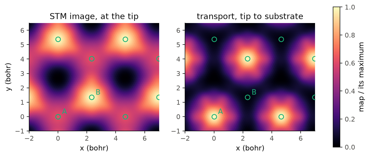
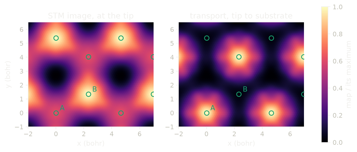
The figure shows the two maps of the bilayer on the same plane, each divided by its maximum. The STM image is brightest on B, with A at 0.61 of it. The transport map is the opposite: it is brightest on A, and B has only 0.029 of the maximum. You can think of it as a question of the path. A sits on an atom of the lower layer, and this is the strong bond between the two layers, so an electron that enters at A goes down to the second layer and into the substrate. B is bright for the tip, but its states do not carry the current through the second layer. So a conductive tip on a bilayer sees the other sublattice than a normal STM does.

Code of this figure (docs/figures/stm_transport/)

compute.py

"""Vertical transport through graphene and bilayer graphene, against the STM image."""
import numpy as np
from defuqumat import Calculator
from common import PSEUDO, save

# one sheet at 0.5 of c: the substrate plane below it, the tip plane above it
graphene = Calculator.from_file("graphene.in", pseudo_dir=PSEUDO)
one = graphene.get_vertical_transport(exit_height=0.38, height=0.62, shape=(30, 30),
                                      broadening=0.02, grid=(6, 6, 1), nbnd=20)
one_stm = graphene.get_stm(height=0.62, shape=(30, 30), width=0.02,
                           grid=(6, 6, 1), nbnd=20)

# two sheets at 0.325 and 0.675 of c
bilayer = Calculator.from_file("graphite.in", pseudo_dir=PSEUDO)
two = bilayer.get_vertical_transport(exit_height=0.14, height=0.86, shape=(30, 30),
                                     broadening=0.02, grid=(6, 6, 1), nbnd=24)
two_stm = bilayer.get_stm(height=0.86, shape=(30, 30), width=0.02,
                          grid=(6, 6, 1), nbnd=24)

save(xy=two.coordinates, transport=two.image, stm=two_stm.values,
     incoherent=two.incoherent,
     corr_one=np.corrcoef(one.image.ravel(), one_stm.values.ravel())[0, 1],
     corr_two=np.corrcoef(two.image.ravel(), two_stm.values.ravel())[0, 1])

plot.py

"""Bilayer graphene: the STM image against the vertical transport map."""
import numpy as np
import style

d = np.load("data.npz")
xy = d["xy"]
n = xy.shape[0]
a1, a2 = n * (xy[1, 0] - xy[0, 0]), n * (xy[0, 1] - xy[0, 0])
f = np.arange(n + 1) / n                      # one cell, both edges included
x = f[:, None] * a1[0] + f[None, :] * a2[0]
y = f[:, None] * a1[1] + f[None, :] * a2[1]
atoms = {"A": (0, 0), "B": (2 / 3, 1 / 3)}


def draw():
    fig, axes = style.figure(2)
    for ax, key, title in zip(axes, ["stm", "transport"],
                              ["STM image, at the tip", "transport, tip to substrate"]):
        field = np.pad(d[key] / d[key].max(), ((0, 1), (0, 1)), mode="wrap")
        for i in range(-1, 3):
            for j in range(-1, 3):
                shift = i * a1 + j * a2
                m = ax.pcolormesh(x + shift[0], y + shift[1], field, shading="gouraud",
                                  cmap=style.CMAP, vmin=0.0, vmax=1.0)
        for name, (f1, f2) in atoms.items():
            for i in range(-1, 3):
                for j in range(-1, 3):
                    p = (f1 + i) * a1 + (f2 + j) * a2
                    ax.plot(*p, "o", mfc="none", mec=style.color(2), ms=7, mew=1.2)
            p = f1 * a1 + f2 * a2
            ax.annotate(name, p, color=style.color(2), xytext=(6, 4),
                        textcoords="offset points", fontsize=11)
        ax.set_xlim(-2.0, 7.0)
        ax.set_ylim(-1.0, 6.5)
        ax.set_aspect("equal")
        ax.set_xlabel("x (bohr)")
        ax.set_title(title)
    axes[0].set_ylabel("y (bohr)")
    style.colorbar(fig, m, list(axes), "map / its maximum")
    return fig


style.main(draw)

Which k-points the current comes from

Let us now make the tip a plane too, parallel to the surface. The map in real space is then gone, and what is left is one weight per k-point, which says from which part of the Fermi surface the electrons tunnel:

\[ W(\mathbf k) = w_{\mathbf k}\, \mathrm{Tr}\!\left[ D_{\mathbf k}\, S^{\rm exit}_{\mathbf k}\, D_{\mathbf k}\, S^{\rm tip}_{\mathbf k} \right], \qquad \sum_{\mathbf k} W(\mathbf k) = \int_{\rm tip} T(\mathbf r)\, d^2 r , \]

with \(S_{\mathbf k}[n, m] = \int_{\rm plane}\psi^{*}_{n\mathbf k}\psi_{m\mathbf k}\,d^2 r\) the overlap of two bands on a plane and \(D_{\mathbf k}\) the diagonal of the on-shell amplitudes \(\sqrt{\tilde\delta(E - \varepsilon_{n\mathbf k})}\). A state with in-plane momentum \(\mathbf k_\parallel\) decays into the vacuum as \(e^{-\sqrt{\kappa_0^2 + k_\parallel^2}\,z}\), so the states far from \(\Gamma\) reach the tip and the substrate less, and a part of the Fermi surface can be large and still carry little current. This is what a momentum-resolved tunnelling experiment sees. We compute it with calc.get_momentum_transport(), here for a square sheet of hydrogen:

sheet = Calculator.from_file("docs/figures/stm_momentum/h-sheet.in",
                             pseudo_dir="tests/data/pseudo")
run = sheet.get_momentum_transport(exit_height=0.3, height=0.7, grid=(32, 32, 1),
                                   broadening=0.03)

k = run.kpoints[:, :2] - np.round(run.kpoints[:, :2])     # into the zone, in 2 pi/a
share = run.shares(np.linalg.norm(k, axis=1) > 0.43)       # near the X points
print(f"near X: {share['bare']:.3f} of the Fermi surface, {share['weight']:.3f} of the current")
print(f"suppression {share['suppression']:.2f}")

near X: 0.246 of the Fermi surface, 0.189 of the current
suppression 1.30

In the outer part of the zone, near the X points, there is 24.6% of the Fermi surface but only 18.9% of the current, so these states tunnel 1.30 times less than their share of the Fermi surface. The reason is their larger \(|\mathbf k_\parallel|\), which makes them decay faster into the vacuum on both sides of the sheet.

get_momentum_transport takes the same exit_height, broadening, grid, spin and polarization as get_vertical_transport, and height can be a list of heights, which costs one band calculation for all of them. Four columns come back, one value per k-point of the full grid: run.weight is \(W(\mathbf k)\), run.tersoff_hamann is the same with a structureless substrate, the local density of states on the tip plane, run.bare is the Fermi surface itself, \(\sum_n \tilde\delta(E - \varepsilon_{n\mathbf k})\), and run.incoherent is every band tunnelling alone. run.as_grid("weight") puts a column on the Monkhorst-Pack grid for a picture of the zone, and run.shares(mask) gives the share of each column in a region of the zone.

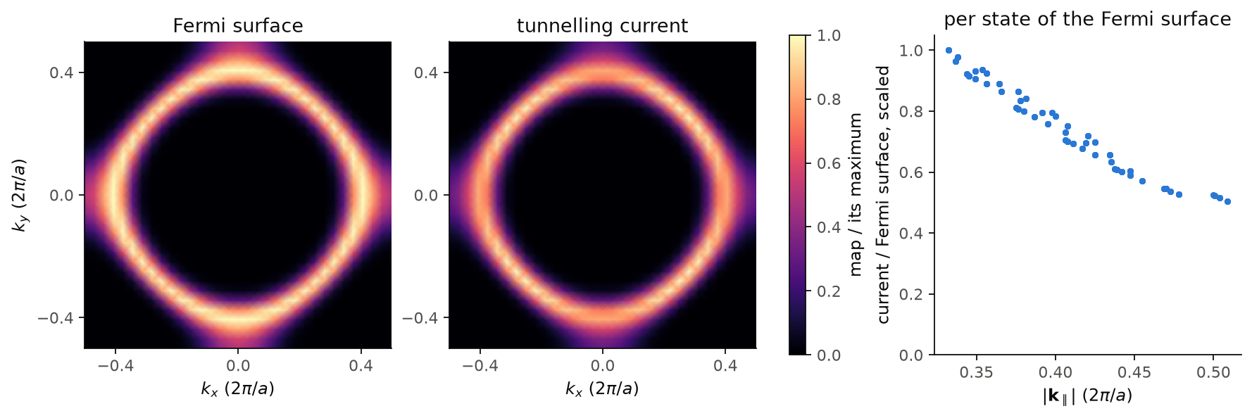
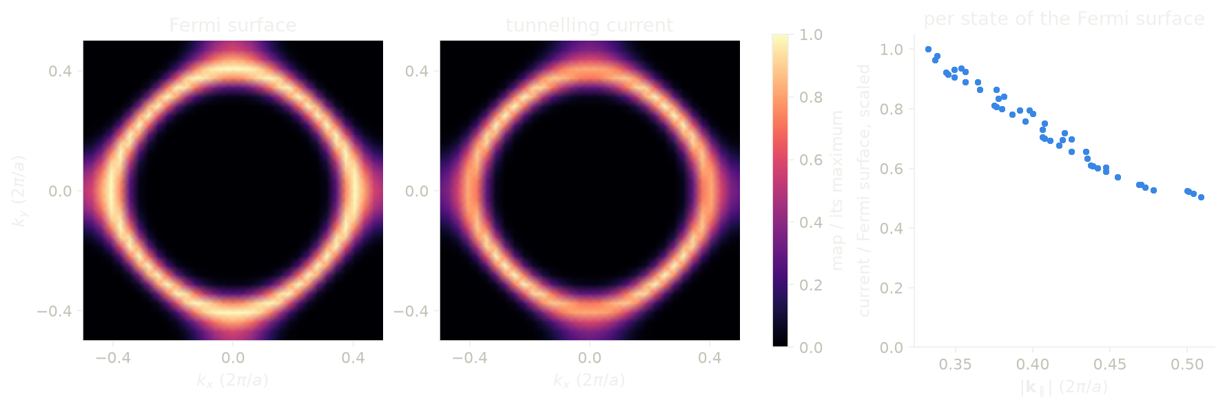
On the left we see the Fermi surface of the sheet, a rounded square around \(\Gamma\), with the most weight near the X points, where the band is flat. In the middle we see the current that tunnels through, which has more weight on the diagonals instead. On the right we divide the two, k-point by k-point: the current per state of the Fermi surface falls by a factor of 2 between \(|\mathbf k_\parallel| = 0.33\) and \(0.51\), in units of \(2\pi/a\). This is the factor \(e^{-\sqrt{\kappa_0^2 + k_\parallel^2}\,z}\) at work, for the tip and for the substrate, each 3 bohr from the sheet. The mesh is \(32\times32\times1\) with a broadening of 0.03 Ry.

Code of this figure (docs/figures/stm_momentum/)

compute.py

"""Which k-points the tunnelling current through a hydrogen sheet comes from."""
from defuqumat import Calculator
from common import PSEUDO, save

calc = Calculator.from_file("h-sheet.in", pseudo_dir=PSEUDO)

# the sheet is at 0.5 of c = 15 bohr: the substrate 3 bohr below, the tip 3 bohr above
run = calc.get_momentum_transport(exit_height=0.3, height=0.7, grid=(32, 32, 1),
                                  broadening=0.03)

save(k=run.kpoints, weight=run.as_grid("weight"), bare=run.as_grid("bare"),
     tersoff_hamann=run.as_grid("tersoff_hamann"))

plot.py

"""The Fermi surface of a hydrogen sheet, and the part of it that tunnels."""
import numpy as np
import style

d = np.load("data.npz")


def zone(name):
    """A column on the grid, with Gamma in the middle and both zone edges."""
    field = np.fft.fftshift(d[name][:, :, 0])
    return np.pad(field, ((0, 1), (0, 1)), mode="wrap")


bare, weight = zone("bare"), zone("weight")
n = bare.shape[0] - 1
k = (np.arange(n + 1) - n // 2) / n
# the current per state, on the k-points of the Fermi surface
kxy = d["k"][:, :2] - np.round(d["k"][:, :2])
size = np.linalg.norm(kxy, axis=1)
b, w = d["bare"].ravel(), d["weight"].ravel()
on = b > 0.2 * b.max()


def draw():
    fig, axes = style.figure(3, layout="constrained")
    for ax, field, title in zip(axes, [bare, weight], ["Fermi surface", "tunnelling current"]):
        m = ax.pcolormesh(k, k, (field / field.max()).T, shading="gouraud",
                          cmap=style.CMAP, vmin=0.0, vmax=1.0)
        ax.set_aspect("equal")
        ax.set_xticks([-0.4, 0.0, 0.4])
        ax.set_yticks([-0.4, 0.0, 0.4])
        ax.set_xlabel(r"$k_x$ ($2\pi/a$)")
        ax.set_title(title)
    axes[0].set_ylabel(r"$k_y$ ($2\pi/a$)")
    style.colorbar(fig, m, list(axes[:2]), "map / its maximum")

    ratio = w[on] / b[on]
    c = axes[2]
    c.plot(size[on], ratio / ratio.max(), "o", color=style.color(0), ms=3)
    c.set_ylim(0.0, 1.05)
    c.set_xlabel(r"$|\mathbf{k}_\parallel|$ ($2\pi/a$)")
    c.set_ylabel("current / Fermi surface, scaled")
    c.set_title("per state of the Fermi surface")
    return fig


style.main(draw)

Limits

The STM image of a spin spiral works for the charge, which is periodic in the cell. A spin-resolved image of a spiral gives an error, because the moment turns from cell to cell, and so does a denser grid. A run with a fixed total magnetization (tot_magnetization) gives an error, because it has one Fermi level per spin and a tip sees one energy. A run in an applied magnetic field also gives an error, because the energy of the field is not in the total, so its Fermi level is not the one of the run without the field. A magnetic tip gives an error on a run with no magnetization, and a tip direction across the axis of a collinear run also gives an error, because such a run has no transverse magnetization, which is not the same as a zero one.

A constant-current scan longer than the period of the cell along the normal gives an error, because there the tip meets the next copy of the surface. A point where the tip never reaches the set-point comes back as nan, with a warning that says how many points. At zero bias the image of an insulator is zero, because the delta sits in the gap, and the code warns about it, so for an insulator you give a bias. All four calculations of this page work with K_POINTS gamma. They agree with an explicit \(k = 0\) to 1e-7, which is what two SCFs at conv_thr = 1e-15 agree to.

The tunnelling spectrum gives the same errors as the image, and two more, because here \(\psi(\mathbf r)\) is sampled and squared at the tip. On a symmetry-reduced k-mesh the spectrum at each tip point is averaged over the images of the point under the symmetry operations, so it is the same as on the full mesh. A reduced k-mesh still gives an error for a magnetic run, for nspin = 2 and for a spinor, which have not been checked, and for a shifted mesh, which the group does not map onto itself. There you pass grid, which builds the full mesh, or run with nosym. A tip inside the augmentation sphere of an ultrasoft or PAW atom gives an error, because there the pseudo-wavefunction is not the true one. So the tip has to be farther from every atom than the augmentation radius, and in practice this means in the vacuum above a surface. On a dense bulk crystal with these datasets every tip position gives an error, because the layers are closer together than that radius (2.4 bohr for SiC), and this is the expected answer, since a tip belongs above a surface. An ultracell already needs nosym, so the error for a symmetry-reduced k-mesh never applies to it. The augmentation-sphere error does apply, to its image, its spectrum and its transmission, and we check it on the atoms of the unit cell, which are the same in every copy. A bias together with energies gives an error, since sts.current is already that window, and the constant-current mode gives an error, since a tip that moves while the bias is swept is a different experiment. sts.current gives an error if the step of the energy axis is larger than width, because the integral would then be wrong by orders of magnitude, not by a few per cent. For a run with no Fermi level, the zero of bias is the middle of the gap, with a warning, and if the run has no gap either, sts.current gives an error.

The vertical transport gives an error for a k-mesh with more than one point along the stacking axis, because the momentum along the normal is not conserved and two such points interfere with a phase that depends on where the substrate plane is. A symmetry-reduced k-mesh gives an error, because a mirror through the slab exchanges the tip and the substrate, and grid builds the full mesh. The substrate plane is always a lattice plane, set by exit_height, while the tip plane may be tilted. A tip or a substrate plane inside an augmentation sphere of an ultrasoft or PAW atom gives an error, and in the vacuum these datasets need nothing extra. A magnetic tip or a magnetic substrate gives an error on a run with no magnetization, and a direction across the axis of a collinear run gives an error for both. A spin spiral gives an error, because the spectrum samples each state on one plane-wave list, and so do a fixed tot_magnetization and an applied field, as for the image. A bias window whose energy step is larger than broadening gives an error, since the current would be wrong by orders of magnitude, and the error says which nenergies is enough. If the atoms are not between the two planes, the code warns. The tip is an s-wave tip, the substrate is infinite and flat, and the map has no absolute scale, because the couplings of the tip and of the substrate are unknown constants.

The momentum-resolved transport gives the same errors as the vertical transport for the k-mesh, the two planes and the substrate, and the code warns if both planes are on the same side of the slab. It has no magnetic tip (tip_spin), because a magnetic plane tip mixes the two spinor components in a way the integral over the plane does not reduce, so for a magnetic tip you use the map of get_vertical_transport. The tip plane is always parallel to the layers, given by height. The weights have no absolute scale, so run.shares() gives shares of a total.

The notebooks for this page are 40, STM images and 41, vertical transport.