Optical spectra

In this page we compute how a crystal absorbs light. We start with the absorption spectrum of an insulator from time-dependent density-functional theory (TDDFT), where an exchange-correlation kernel decides how the excited electron and the hole it leaves behind interact. Then we compute the whole optical conductivity tensor of a magnetic metal, and from its off-diagonal part the Kerr rotation of the light it reflects.

The absorption spectrum

What does an optical absorption experiment measure? It measures the imaginary part of the macroscopic dielectric function, \(\mathrm{Im}\,\epsilon_M(\omega)\), which is also what ellipsometry gives. We build it in two steps. The first is the response of independent Kohn-Sham electrons, as a matrix in the reciprocal lattice vectors \(\mathbf G\):

\[ \chi^0_{\mathbf G\mathbf G'}(\omega) = \frac{1}{\Omega}\sum_{\mathbf k}\sum_{ij} \frac{(f_i-f_j)\,\rho^{ij}_{\mathbf G}\,\rho^{ij*}_{\mathbf G'}} {\epsilon_i-\epsilon_j+\omega+i\eta}, \qquad \rho^{ij}_{\mathbf G}=\langle u_i|e^{-i\mathbf G\cdot\mathbf r}|u_j\rangle . \]

This is a sum over pairs of occupied and empty bands, so it needs empty bands, and \(\eta\) is the broadening of every peak. The second step is a Dyson equation, which adds the Coulomb interaction \(v\) and the exchange-correlation kernel \(f_{xc}\):

\[ \epsilon^{-1} = 1 + X\left(1 - X - \tilde f_{xc}X\right)^{-1}, \qquad X = v^{1/2}\chi^0 v^{1/2}, \qquad \tilde f_{xc} = v^{-1/2} f_{xc} v^{-1/2}, \qquad \epsilon_M(\omega) = \frac{1}{\left[\epsilon^{-1}(\omega)\right]_{00}} . \]

The macroscopic dielectric function is the inverse of the head of \(\epsilon^{-1}\), meaning that the other elements of the matrix, the local fields, enter \(\epsilon_M\) through the inversion. With \(f_{xc}=0\) the result is the random-phase approximation (RPA). The kernel is what can bind an electron-hole pair into an exciton, and here the question is how strong the kernel is at long wavelength. We measure it with one number,

\[ \alpha = -4\pi\,[\tilde f_{xc}]_{00} . \]

This is the \(\alpha\) of the long-range kernel \(f_{xc}=-\alpha/q^2\) that has the same head as our kernel. In ALDA the kernel is finite at \(\mathbf q = 0\) while \(v\) diverges, so \(\alpha\) is exactly zero, and no adiabatic local kernel can bind an exciton however strong it is. The bootstrap kernel of Sharma, Dewhurst, Sanna and Gross,

\[ f^{\rm BS}_{xc} = -\,\frac{\epsilon^{-1}(\mathbf q,0)\,v(\mathbf q)}{\epsilon_0(\mathbf q,0)-1}, \qquad \epsilon_0 = 1 - v\chi^0 , \]

goes as \(1/q^2\), so its \(\alpha\) is not zero. It has no free parameter, and since it depends on \(\epsilon^{-1}\) itself, the kernel and the Dyson equation are solved together until they agree. Here we take silicon in LDA on a \(4\times4\times4\) grid, and we compute its spectrum with calc.get_absorption():

import numpy as np
from defuqumat import Calculator

silicon = Calculator.from_file("docs/figures/optics_absorption/si.in",
                               pseudo_dir="tests/data/pseudo")
omega = np.arange(0.0, 0.60, 0.004)          # Ry
spectrum = silicon.get_absorption(omega, kernel="bootstrap", nbnd=60,
                                  ecut_response=8.0, broadening=0.012)

print(f"alpha = {spectrum.alpha:+.4f} after {spectrum.iterations} passes")
print(f"eps_M(0) in RPA = {spectrum.static_rpa:.3f}, "
      f"band truncation {spectrum.static_residual:+.4f}")
peak = np.argmax(spectrum.absorption)
print(f"largest Im eps_M = {spectrum.absorption[peak]:.2f} "
      f"at {spectrum.frequencies_ev[peak]:.2f} eV")

alpha = +0.0232 after 9 passes
eps_M(0) in RPA = 22.332, band truncation -0.0129
largest Im eps_M = 79.18 at 3.76 eV

The bootstrap kernel converged in 9 passes, and its long-range strength is \(\alpha = +0.0232\). The second line is a check on the number of empty bands, which is the one error of a sum over states that gives no visible symptom. The band truncation is \(\epsilon_M(0)\) of this run in RPA minus the same quantity from the static linear response, which needs no empty bands at all, so the sum over 60 bands is 0.013 below the complete value, and nbnd is what makes the difference smaller. The value 22.33 itself is far from the measured dielectric constant of silicon, 11.7. A converged LDA calculation gives about 13 to 14, already above 11.7, so most of the distance to 22.33 comes from this \(4\times4\times4\) grid, which is too coarse even for the static limit, and you should read the spectra below as a demonstration of the method rather than as converged numbers. The largest absorption is at 3.76 eV, below the measured \(E_2\) peak of silicon at 4.25 eV, and 64 k-points give a spectrum made of separate peaks of width \(\eta\) rather than a smooth curve.

The keywords of get_absorption are:

• frequencies: the photon energies, in Ry. This is the one argument you must give.
• kernel: "rpa", "alda", "lrc", "bootstrap" or "bootstrap-1". "lrc" is the long-range kernel \(f_{xc} = -\alpha/q^2\) and needs alpha=, an empirical number for each material. "bootstrap-1" is the bootstrap evaluated once from the RPA \(\epsilon^{-1}\), with no iteration.
• nbnd: the number of bands of the sum over states. If you do not give it, the code takes four times the number of occupied bands.
• ecut_response: the cutoff in Ry of the \(\mathbf G\) vectors of the matrix \(\chi^0_{\mathbf G\mathbf G'}\). Too small a value leaves out the local fields, and the cost grows as its square.
• broadening: \(\eta\) in Ry, the width of every peak.
• scissor: a rigid shift of the empty bands in Ry, which corrects the LDA gap. It is applied to the energies and to the velocity matrix elements.
• kpoints: a denser full k-grid for the spectrum than the one of the SCF. It can be the whole grid or its irreducible wedge.

spectrum.absorption is \(\mathrm{Im}\,\epsilon_M\) averaged over the three directions, on spectrum.frequencies_ev. spectrum.epsilon is the whole complex \(3\times3\) tensor at each frequency, and spectrum.epsilon_no_local_fields is the same without the local fields. spectrum.plot() draws the spectrum.

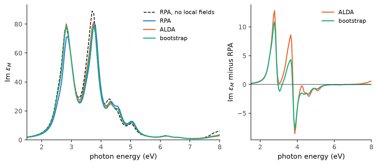
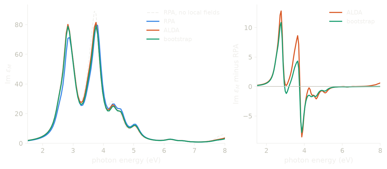
On the left we see the spectrum of silicon with three kernels, on the same \(\chi^0\), and in the right panel the difference of each kernel to RPA. We see two peaks, at 2.8 and 3.76 eV, which are the \(E_1\) and \(E_2\) peaks of silicon, both below the measured 3.4 and 4.25 eV because of the LDA gap. The dashed curve is RPA without the local fields, and the local fields take its \(E_2\) peak down from 89.0 to 80.1, about 10%. Both kernels are attractive, so they move oscillator strength down in energy, from \(E_2\) to \(E_1\), and the first moment of the spectrum goes from 3.648 eV in RPA to 3.592 eV with ALDA and 3.587 eV with the bootstrap. The bootstrap raises the \(E_1\) peak by up to 10.9 and ALDA by up to 12.8, so on this plot ALDA moves about as much weight as the bootstrap does. Silicon has only a weakly bound exciton, of about 15 meV, far below the broadening here, so there is no peak below the gap for either kernel to create. The difference between the two is the number \(\alpha\), exactly zero for ALDA and \(+0.0232\) for the bootstrap, and it decides what happens in a crystal where the electron-hole attraction is strong enough to bind a pair below the gap.

Code of this figure (docs/figures/optics_absorption/)

compute.py

"""The absorption spectrum of silicon with three kernels: RPA, ALDA and the bootstrap."""
import numpy as np
from defuqumat import Calculator
from common import PSEUDO, save

calc = Calculator.from_file("si.in", pseudo_dir=PSEUDO)
omega = np.arange(0.0, 0.60, 0.004)      # Ry

out = {}
for kernel in ("rpa", "alda", "bootstrap"):
    s = calc.get_absorption(omega, kernel=kernel, nbnd=60, ecut_response=8.0,
                            broadening=0.012)
    out[kernel] = s.absorption
    out[kernel + "_alpha"] = s.alpha
    out[kernel + "_passes"] = s.iterations
    out[kernel + "_residual"] = s.static_residual
    if kernel == "rpa":
        eps = s.epsilon_no_local_fields
        out["rpa_no_local_fields"] = np.mean([eps[:, i, i].imag for i in range(3)], axis=0)

save(energy=s.frequencies_ev, **out)

plot.py

"""Silicon: Im eps_M with three kernels, and what each kernel changes."""
import numpy as np
import style

d = np.load("data.npz")
e = d["energy"]
kernels = [("rpa", "RPA"), ("alda", "ALDA"), ("bootstrap", "bootstrap")]


def draw():
    fig, (a, b) = style.figure(2, gridspec_kw={"width_ratios": [1.6, 1]})
    a.plot(e, d["rpa_no_local_fields"], **style.reference(),
           label="RPA, no local fields")
    for k, (name, label) in enumerate(kernels):
        a.plot(e, d[name], color=style.color(k), label=label)
        if name != "rpa":
            b.plot(e, d[name] - d["rpa"], color=style.color(k), label=label)
    a.set_xlim(1.5, 8.0)
    a.set_ylim(bottom=0.0)
    a.set_xlabel("photon energy (eV)")
    a.set_ylabel(r"Im $\epsilon_M$")
    a.legend(loc="upper right")
    style.zero_line(b)
    b.set_xlim(1.5, 8.0)
    b.set_xlabel("photon energy (eV)")
    b.set_ylabel(r"Im $\epsilon_M$ minus RPA")
    b.legend(loc="upper right")
    return fig


style.main(draw)

The optical conductivity

We now go to a metal, and to the whole tensor of the optical conductivity, which is the current along \(i\) that a field along \(j\) at frequency \(\omega\) drives. In the independent-particle picture it is a sum over pairs of bands, plus the Drude term of the carriers at the Fermi level:

\[ \sigma_{ij}(\omega) = \frac{i}{\Omega}\sum_{\mathbf k}\sum_{n,m} \frac{W_n\,(1-f_m)}{\epsilon_{mn}} \left[\frac{v^i_{nm}v^j_{mn}}{\omega-\epsilon_{mn}+i\eta} + \frac{\overline{v^i_{nm}v^j_{mn}}}{\omega+\epsilon_{mn}+i\eta}\right] + \frac{\omega_{p,ij}^2}{4\pi(\gamma - i\omega)}, \qquad \omega_{p,ij}^2 = \frac{4\pi}{\Omega}\sum_{\mathbf k} w_{\mathbf k}\sum_n v^i_{nn}\,v^j_{nn}\,\delta(\epsilon_{n\mathbf k} - E_F) . \]

Here \(v = \partial H/\partial\mathbf k\) is the velocity operator, which includes the nonlocal part of the pseudopotential, \(\epsilon_{mn}\) is the energy of the transition and \(\omega_p\) is the plasma frequency, a Fermi-surface average of the squared band velocity. \(W_n\) is the occupation of band \(n\) times its k weight, \(f_m\) the occupation of band \(m\), and \(\gamma\) the relaxation rate of the Drude term. The diagonal part, \(\mathrm{Re}\,\sigma_{xx}\), is the normal absorption of the metal, and the optical constants that reflectivity and ellipsometry measure follow from it through \(\epsilon_{ij}(\omega) = \delta_{ij} + 4\pi i\sigma_{ij}/\omega\).

The antisymmetric part, \(\sigma_{xy} = -\sigma_{yx}\), is different. Time reversal makes it zero, so a crystal with no magnetic order has none, however heavy its atoms are. A collinear magnet without spin-orbit coupling has none either, because a spin rotation combined with time reversal is still a symmetry. So \(\sigma_{xy}\) needs magnetism and spin-orbit coupling together, and fcc nickel has both. Its static limit, taken with \(\eta \to 0\) first, is the anomalous Hall conductivity, the transverse current that flows with no applied magnetic field. Here we take nickel with spin-orbit coupling and the moment along \(z\), on a \(4\times4\times4\) grid, and we compute the tensor with calc.get_optical_conductivity():

nickel = Calculator.from_file("docs/figures/optics_kerr/ni-soc.in",
                              pseudo_dir="tests/data/pseudo")
sigma = nickel.get_optical_conductivity(nbnd=36, window=0.6, nw=200,
                                        broadening=0.01)

ev = sigma.frequencies_ev
s = sigma.sigma_s_per_cm                     # (frequency, 3, 3), S/cm
i = np.argmin(abs(ev - 1.0))
print(f"at {ev[i]:.2f} eV: sigma_xx = {s[i, 0, 0].real:8.1f} S/cm")
print(f"           sigma_xy = {s[i, 0, 1].real:8.1f} S/cm")
print(f"gap at the band cut {sigma.band_cut_gap:.4f} Ry, "
      f"{sigma.degenerate_pairs} pairs dropped")

at 0.98 eV: sigma_xx =   2917.3 S/cm
           sigma_xy =   -139.4 S/cm
gap at the band cut 0.0054 Ry, 0 pairs dropped

At 1 eV the off-diagonal conductivity is about 5% of the diagonal one, and this small ratio is the reason a Kerr angle is a fraction of a degree. The last line says that the sum over 36 bands stops at a gap of 0.0054 Ry and that no pair of bands was dropped as degenerate. The conductivity is a fixed-density calculation with empty bands on top of the SCF, on the k-points of the SCF unless you give others. Note that 64 k-points are far too few for a metal, so these two numbers are not converged, and in the next section we see by how much.

The keywords of get_optical_conductivity are:

• nbnd: the number of bands. If you do not give it, the code takes three times the number of occupied bands.
• window, nw: the frequency grid, from zero to window Ry in nw points. The first point is \(\omega = 0\), which is what sigma.hall_conductivity reads.
• frequencies: your own frequencies in Ry, in place of window and nw.
• broadening: \(\eta\) in Ry, the width of every interband transition.
• relaxation: \(\gamma\) in Ry of the Drude term. If you do not give it, the code takes broadening.
• intraband: False leaves out the Drude term.
• scissor: a rigid shift of the empty bands in Ry.
• kpoints: a denser full grid for the sum, in place of the grid of the SCF. It can be the whole grid or its irreducible wedge.
• fermi_energy: the Fermi level in Ry. With a denser grid you give the one of the SCF, fermi_energy=scf.fermi_energy, so the occupations stay those of the ground state.
• method: "frequency", the default, or "curvature". "frequency" gives the whole spectrum, and its value at \(\omega = 0\) is the conductivity at the finite broadening \(\eta\), which is what a measured spectrum goes to at zero frequency. "curvature" gives only \(\omega = 0\), as the Berry-curvature integral with \(\eta \to 0\), which is the intrinsic anomalous Hall conductivity. For an insulator the two are the same, and for a metal they are not.
• degeneracy_tol: the gap in Ry below which an occupied and an empty band count as degenerate, so their pair is dropped. The Limits note below says how the code chooses it when you do not give it.

sigma.sigma_s_per_cm is the complex tensor in S/cm with the shape (frequency, 3, 3), and sigma.sigma the same in atomic units. sigma.dielectric is \(\epsilon_{ij}(\omega)\), sigma.plasma_ev is the \(3\times3\) tensor \(\hbar\omega_p\) in eV, and sigma.hall_conductivity is the antisymmetric part at \(\omega = 0\) in S/cm, which is the intrinsic anomalous Hall conductivity only with method="curvature".

The Kerr angle

Let us now ask what \(\sigma_{xy}\) does to light. Linearly polarized light reflected at normal incidence from a magnet with its moment along \(z\) comes back rotated by a small angle \(\theta_K\) and with a small ellipticity \(\eta_K\), which is the polar magneto-optical Kerr effect. Both come from the conductivity tensor alone:

\[ \theta_K + i\,\eta_K = \frac{-\sigma_{xy}} {\sigma_{xx}\sqrt{1 + 4\pi i\,\sigma_{xx}/\omega}} . \]

So nothing new is computed for the Kerr angle, and sigma.kerr gives it in degrees at each frequency. The Kerr rotation is what a magneto-optical microscope measures to image the domains of a magnetic film. Note that the expression divides by \(\sigma_{xx}\), so it becomes large wherever \(\sigma_{xx}\) is small. Here we read it in the visible, with the sigma of nickel from above:

kerr = sigma.kerr                            # theta_K + i eta_K, degrees
visible = (ev > 1.5) & (ev < 3.5)
j = np.argmax(np.where(visible, abs(kerr.real), 0.0))
print(f"largest rotation in 1.5 to 3.5 eV: {kerr.real[j]:+.3f} deg at {ev[j]:.2f} eV")
print(f"ellipticity there: {kerr.imag[j]:+.3f} deg")

largest rotation in 1.5 to 3.5 eV: +1.031 deg at 1.85 eV
ellipticity there: -0.902 deg

Is this number converged? A metal has a Fermi surface, and both the Drude term and the static Hall conductivity are integrals over it, so they need many more k-points than an insulator does. In the figure we repeat the same calculation on the whole \(4\times4\times4\), \(6\times6\times6\) and \(8\times8\times8\) grids, with the Fermi level of the SCF and the same 36 bands and \(\eta = 0.01\) Ry. Each denser grid is the whole Monkhorst-Pack grid, which is what KPoints.automatic() gives when we pass it no symmetry operations:

from defuqumat.system.kpoints import KPoints

cell = nickel.system.cell
mesh = KPoints.automatic((8, 8, 8), (0, 0, 0), cell, precision=cell.precision)
print(f"{len(mesh.weights)} k-points")

512 k-points

and we give it as kpoints=mesh, with fermi_energy=scf.fermi_energy where scf = nickel.get_scf(). The figure takes 12 minutes on one core, most of it on the \(8\times8\times8\) grid of 512 k-points.

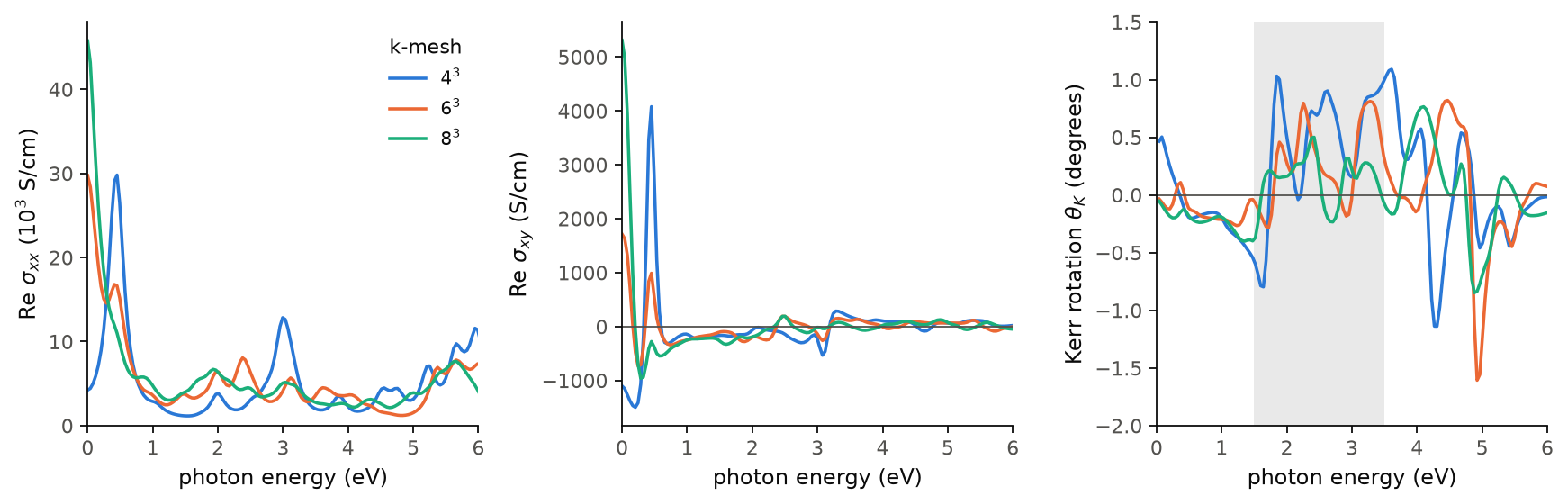
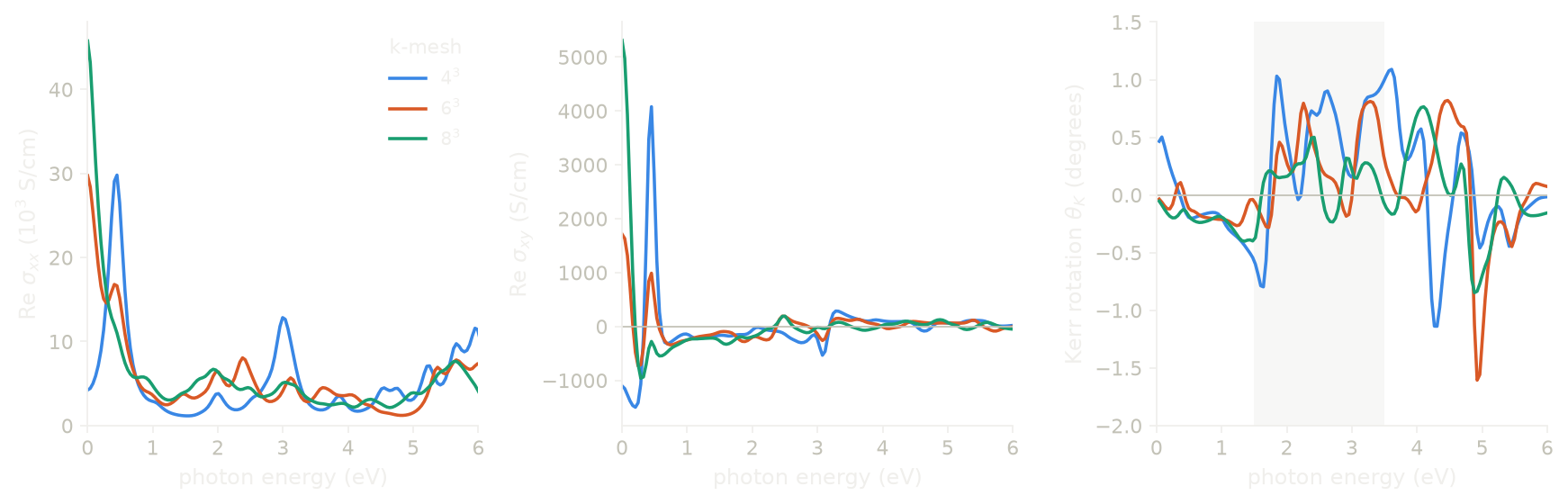
The SCF gives a moment of \(0.617\,\mu_B\) along \(z\). On the left we see \(\mathrm{Re}\,\sigma_{xx}\), and the Drude peak at \(\omega = 0\) grows with the mesh, because the plasma frequency \(\hbar\omega_p\) goes from 0.85 eV to 4.42 eV and then 5.74 eV, which means that the Fermi surface is not converged even on 512 k-points. In the middle panel we see \(\mathrm{Re}\,\sigma_{xy}\), and its static value at \(\eta = 0.01\) Ry is \(-1103\), \(+1713\) and \(+5310\) S/cm on the three meshes, so it changes sign and then grows. The static Hall conductivity of nickel is a sum dominated by a few k-points where two bands are almost degenerate at the Fermi level, and a converged value needs meshes much denser than these, so you should not read any of the three numbers as the Hall conductivity of nickel. Above about 1 eV the three curves of \(\sigma_{xy}\) come closer, because there the interband transitions spread over the whole zone. On the right we see the Kerr rotation, and in the visible, the grey band, it stays within about 1 degree of zero, but its shape still moves with the mesh. The largest rotation in the visible is \(+1.03\) degrees at 1.85 eV on \(4\times4\times4\), \(+0.81\) at 3.28 eV on \(6\times6\times6\) and \(+0.50\) at 2.42 eV on \(8\times8\times8\), and the curve changes by up to 0.59 degrees between the last two meshes. The measured rotation of bulk nickel in the visible is about 0.1 degree, so all three meshes give a rotation several times too large, and the spectrum is not converged. A converged one needs a denser grid than we can show here.

Code of this figure (docs/figures/optics_kerr/)

compute.py

"""The optical conductivity and the Kerr angle of fcc nickel, on three k-meshes."""
from defuqumat import Calculator
from defuqumat.system.kpoints import KPoints
from common import PSEUDO, save

calc = Calculator.from_file("ni-soc.in", pseudo_dir=PSEUDO)
scf = calc.get_scf()
cell = calc.system.cell

out = {"moment": scf.magnetization_vector[2]}
for n in (4, 6, 8):
    mesh = KPoints.automatic((n, n, n), (0, 0, 0), cell, precision=cell.precision)
    sigma = calc.get_optical_conductivity(kpoints=mesh, nbnd=36, window=0.6,
                                          nw=200, broadening=0.01,
                                          fermi_energy=scf.fermi_energy)
    s = sigma.sigma_s_per_cm                     # (frequency, 3, 3), S/cm
    out[f"sxx{n}"] = s[:, 0, 0]
    out[f"sxy{n}"] = 0.5 * (s[:, 0, 1] - s[:, 1, 0])
    out[f"kerr{n}"] = sigma.kerr                 # degrees
    out[f"hall{n}"] = sigma.hall_conductivity[0, 1]
    out[f"fsum{n}"] = sigma.fsum
    out[f"plasma{n}"] = sigma.plasma_ev[0, 0]   # hbar omega_p, eV

save(energy=sigma.frequencies_ev, **out)

plot.py

"""Nickel: sigma_xx, sigma_xy and the Kerr rotation on three k-meshes."""
import numpy as np
import style

d = np.load("data.npz")
e = d["energy"]
meshes = [(4, r"$4^3$"), (6, r"$6^3$"), (8, r"$8^3$")]


def draw():
    fig, (a, b, c) = style.figure(3)
    for k, (n, label) in enumerate(meshes):
        a.plot(e, d[f"sxx{n}"].real / 1e3, color=style.color(k), label=label)
        b.plot(e, d[f"sxy{n}"].real, color=style.color(k), label=label)
        c.plot(e[1:], d[f"kerr{n}"].real[1:], color=style.color(k), label=label)
    a.set_ylabel(r"Re $\sigma_{xx}$ ($10^3$ S/cm)")
    a.set_ylim(0.0, None)
    b.set_ylabel(r"Re $\sigma_{xy}$ (S/cm)")
    c.set_ylabel(r"Kerr rotation $\theta_K$ (degrees)")
    for ax in (a, b, c):
        ax.set_xlim(0.0, 6.0)
        ax.set_xlabel("photon energy (eV)")
    for ax in (b, c):
        style.zero_line(ax)
    c.set_ylim(-2.0, 1.5)
    c.axvspan(1.5, 3.5, color=style.ink2(), alpha=0.12, lw=0)
    a.legend(loc="upper right", title="k-mesh")
    fig.tight_layout()
    return fig


style.main(draw)

Limits

The absorption spectrum needs an insulator with fixed occupations. For a metal the sum over pairs of bands has no intraband term, so the Drude part of the response would be missing, and the code gives an error. A state where an empty band carries occupation at some k-point also gives an error. Ultrasoft and PAW datasets give an error, because every matrix element would need the augmentation charge, and so do a noncollinear magnetization, a spin spiral and a Hubbard \(U\). A spinor run without a magnetization works, with or without spin-orbit coupling. On selenium with spin-orbit coupling the static value is 0.27 per cent from the Sternheimer solve at 144 bands and ecut_response = 12. With nspin = 2 the spectrum is the response of the charge, and the alda kernel gives an error if the ground state has a moment, because then the kernel couples the charge to the magnetization. The bootstrap and lrc kernels act on the charge only. The spectrum is at \(\mathbf q = 0\) only, since a finite \(\mathbf q\) needs the states at \(\mathbf k + \mathbf q\).

On a symmetry-reduced k-set both the absorption spectrum and the optical conductivity are averaged over the group the k-set was cut with, so they come out the same as on the whole grid. For the spectrum this rotates the two \(\mathbf G\) indices of \(\chi^0_{\mathbf G\mathbf G'}\) at once, and for the conductivity it makes the antisymmetric part zero when there is time reversal. A magnetic run gives an error on a reduced k-set. So does a shifted mesh, because the group does not map a shifted mesh onto itself. The spectrum also gives an error on a reduced k-set with nspin = 2 or a spinor, because that case has not been checked. Then you pass the whole unshifted grid as kpoints. A shifted whole grid works for the spectrum itself, but the band-truncation check static_residual gives an error on it, so you pass static_residual=False. The absorption spectrum works with K_POINTS gamma. The bands are solved again on the whole sphere, and the spectrum agrees with an explicit \(k = 0\) to 1.4e-9.

The alda kernel gives an error with a gradient-corrected or meta-GGA functional, because the ALDA kernel is local in the density and a GGA kernel is not. The lrc kernel gives an error without alpha. If the bootstrap kernel does not converge, the code gives an error and returns no spectrum, because a spectrum from a kernel still in motion belongs to no functional.

The optical conductivity gives an error for a spin spiral, whose two spinor components live on different spheres. Its Drude term gives an error with tetrahedra, which have no smeared delta function at the Fermi level, so you use smearing, or intraband=False to read the interband part alone. Ultrasoft and PAW datasets work, and so does nspin = 2, where the conductivities of the two spin channels are added. sigma.hall_conductivity gives an error when your frequencies do not start at \(\omega = 0\), since it is the static limit. The anomalous Hall conductivity of a metal needs a very dense k-mesh, as we saw above, so you quote it with its convergence in the k-mesh.

Two numbers come with every conductivity and you should read them. sigma.band_cut_gap is the gap between the last band in the sum and the first band left out. If it is close to zero, the sum stops inside a degenerate set of bands and the result is wrong, so the code warns and you change nbnd. sigma.degenerate_pairs counts the occupied and empty pairs of bands closer in energy than degeneracy_tol (in Ry), which are dropped, and it is normally zero. If you do not give degeneracy_tol, the code takes it from how well the bands were converged, which is 1e-5 Ry at the default conv_thr. A value you give below what the eigensolver resolves is used, and the code warns. With smearing the dropped pairs cancel and change nothing, and the code warns where they do not cancel, which is with fixed occupations and with method="curvature". The same degeneracy_tol works the same way on get_berry_curvature, get_shift_current, get_shg, get_vertical_transport, get_ultracell, get_ultracell_transport and get_scf.

The notebooks for this page are 27, excitons and TDDFT and 30, magneto-optics.