Topology

In this page we compute the geometry of the occupied bands. We start with the Berry curvature, which is a field over the Brillouin zone, then we integrate it to the Chern number of a plane, and finally we compute the \(\mathbb Z_2\) invariant of an insulator with time-reversal symmetry, in two dimensions and in three.

The Berry curvature

We start with the Berry connection of the occupied bands, which says how the periodic part \(u_{n\mathbf k}\) of a Bloch state changes its phase when \(\mathbf k\) moves. Its curl is the Berry curvature:

\[ \mathbf A(\mathbf k) = i \sum_{n\,\rm occ} \langle u_{n\mathbf k}|\nabla_{\mathbf k} u_{n\mathbf k}\rangle, \qquad \Omega(\mathbf k) = \big(\nabla_{\mathbf k}\times\mathbf A\big)_\perp . \]

\(\Omega\) is the component normal to a plane of the zone, so it is a field over that plane, in units of an area (bohr\(^2\)). We compute it from the sum over the empty bands,

\[ \Omega_n(\mathbf k) = -2\,{\rm Im}\sum_{m\neq n} \frac{\langle\psi_n|\partial_{k_1}H|\psi_m\rangle\, \langle\psi_m|\partial_{k_2}H|\psi_n\rangle} {(\varepsilon_n-\varepsilon_m)^2}, \qquad \Omega = \sum_{n\,\rm occ}\Omega_n , \]

which is the Kubo form. For an ultrasoft or PAW dataset the code adds the terms with the \(\mathbf k\) derivative of the overlap operator. The curvature acts on an electron like a magnetic field in \(\mathbf k\) space, so it gives the anomalous velocity, and its integral over the occupied states is the anomalous Hall conductivity. Where it sits in the zone is what the valley Hall effect and circular dichroism in photoemission see.

Symmetry decides a lot here. Time reversal gives \(\Omega(-\mathbf k) = -\Omega(\mathbf k)\) and inversion gives \(\Omega(-\mathbf k) = \Omega(\mathbf k)\), so a crystal with both has zero curvature at every \(\mathbf k\). Here we take AlAs, which has time reversal but no inversion centre, so its curvature is not zero point by point. We compute it with calc.get_berry_curvature():

import numpy as np
from defuqumat import Calculator

alas = Calculator.from_file("docs/figures/topology_berry_map/alas.in",
                            pseudo_dir="tests/data/pseudo")
omega = alas.get_berry_curvature(shape=(24, 24), nbnd=20, method="kubo")
print(omega.curvature.shape)
print(f"max |Omega|    {np.abs(omega.curvature).max():.4f}")
print(f"truncation     {omega.truncation:.4f}")
print(f"sum of the map {omega.chern_number:.2e}")

(24, 24)
max |Omega|    1.3605
truncation     0.0199
sum of the map 2.82e-06

The map has one value at each of the \(24\times24\) points of the plane, and its largest value, 1.3605 in the units of omega.curvature, which here differ from bohr\(^2\) by 0.15%, is of order one, so the curvature of AlAs is not small. The Chern number from this map, omega.chern_number, which is the mean of the map divided by \(2\pi\), is \(2.8\times10^{-6}\), which is close to zero but not zero. Time reversal makes the exact integral zero, and the small rest is there because a sum over a mesh is not an exact integral. We come back to this in the next section. AlAs runs here at 10 Ry on a \(4\times4\times4\) mesh of the SCF, so the map is a picture of the symmetry and not a converged curvature.

The keywords of get_berry_curvature are:

• shape: the mesh of the plane, \((n_1, n_2)\) points along the two crystal directions that span it.
• axis, offset: the crystal direction that is held fixed, and its value. If you do not give them, the plane is \(k_3 = 0\), spanned by \(\mathbf b_1\) and \(\mathbf b_2\).
• method: "kubo" for the map above, or "fhs" for the lattice construction of the next section. If you do not give it, the code uses "fhs".
• nbnd: the number of bands of the Kubo sum. The sum over empty bands stops at nbnd, so you add bands until the truncation is small.
• nocc: the number of occupied bands. If you do not give it, the code divides the number of electrons by two, or by one for a spinor run.

omega.curvature is the map, with shape \((n_1, n_2)\), in units where its mean divided by \(2\pi\) is the Chern number, so you divide it by the area \(|\mathbf b_1\times\mathbf b_2|\) of the plane to have it in bohr\(^2\). omega.curvature_by_band has one more axis for the occupied bands, and omega.truncation is the largest change of the map when the highest empty band is left out, relative to the largest value of the map. Here it is 0.0199, so with 20 bands the last empty band still changes the map by 2%. omega.plot() draws the map.

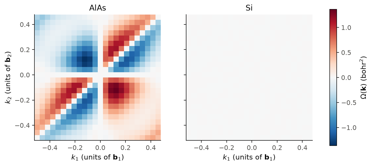
The figure shows the plane \(k_3 = 0\), spanned by \(\mathbf b_1\) and \(\mathbf b_2\), with \(\Gamma\) in the middle, on the \(24\times24\) mesh of the snippet, and both panels have the same color scale. On the left we see AlAs. The curvature reaches 1.36 bohr\(^2\), with the largest values at \((k_1, k_2) = (\pm 1/8, \mp 1/8)\), and each red lobe has a blue lobe at \(-\mathbf k\), so the map is odd, as time reversal requires. This is why the integral is zero while the map is of order one. The white line on the diagonal \(k_1 = k_2\) lies in a mirror plane of zincblende, which changes the sign of \(\Omega\), so away from \(\Gamma\) the curvature there is zero to \(10^{-8}\) bohr\(^2\), and away from \(\Gamma\) on the lines \(k_1 = 0\) and \(k_2 = 0\) it is below 0.003 bohr\(^2\). At \(\Gamma\) itself we get 0.0099 bohr\(^2\), 0.7% of the largest value, where time reversal requires zero, so this is the size of the numerical error of this map. On the right we see silicon, with inversion and time reversal, and its curvature is below \(6\times10^{-8}\) bohr\(^2\) at every point. So silicon has no Berry curvature at all, which is a stronger statement than a zero integral.

Code of this figure (docs/figures/topology_berry_map/)

compute.py

"""The Berry curvature of AlAs and of silicon on the plane k3 = 0."""
import numpy as np
from defuqumat import Calculator
from common import PSEUDO, save

data = {}
for name in ("alas", "si"):
    calc = Calculator.from_file(f"{name}.in", pseudo_dir=PSEUDO)
    omega = calc.get_berry_curvature(shape=(24, 24), nbnd=20, method="kubo")
    b = np.asarray(calc.system.cell.bg)             # b1, b2, b3 in 1/bohr
    area = np.linalg.norm(np.cross(b[0], b[1]))     # the area of the plane
    data[name] = omega.curvature / area             # Omega in bohr^2
    data[name + "_chern"] = calc.get_chern(shape=(24, 24))
    print(name, "max |Omega| %.4f bohr^2, C = %.2e"
          % (np.abs(data[name]).max(), data[name + "_chern"]), flush=True)

save(**data)

plot.py

"""The Berry curvature of AlAs and of silicon, on one color scale."""
import numpy as np
import style

d = np.load("data.npz")


def centred(omega):
    """Roll the mesh so that Gamma is in the middle, k from -1/2 to 1/2."""
    n = omega.shape[0]
    return np.roll(omega, (n // 2, n // 2), axis=(0, 1)), (np.arange(n + 1) - n // 2 - 0.5) / n


def draw():
    fig, axs = style.figure(2, sharey=True)
    limit = np.abs(d["alas"]).max()
    for ax, name, title in zip(axs, ("alas", "si"), ("AlAs", "Si")):
        omega, edges = centred(d[name])
        m = ax.pcolormesh(edges, edges, omega.T, cmap="RdBu_r", vmin=-limit, vmax=limit)
        ax.set_aspect("equal")
        ax.set_title(title, color=style.ink())
        ax.set_xlabel(r"$k_1$ (units of $\mathbf{b}_1$)")
    axs[0].set_ylabel(r"$k_2$ (units of $\mathbf{b}_2$)")
    style.colorbar(fig, m, axs, r"$\Omega(\mathbf{k})$ (bohr$^2$)")
    return fig


style.main(draw)

The Chern number

Let us now integrate the curvature over the plane. The integral is the Chern number:

\[ C = \frac{1}{2\pi}\int_{\rm BZ} \Omega(\mathbf k)\, d^2k \in \mathbb Z . \]

\(C\) is an integer, and it can change only when the gap closes. For a two-dimensional insulator it gives the quantized Hall conductance, \(\sigma_{xy} = C\,e^2/h\), and it counts the chiral edge states. A sum of the Kubo map over a mesh is not an integer, so we compute \(C\) in a different way, with the lattice construction of Fukui, Hatsugai and Suzuki. We take the overlap matrices of the occupied states at neighbouring points of the mesh,

\[ M^{(\mathbf k,\mathbf k')}_{mn} = \langle u_{m\mathbf k}|\hat S|u_{n\mathbf k'}\rangle , \qquad C = \frac{1}{2\pi}\sum_{\square} \arg\Big[\det M^{(\mathbf k,\mathbf k+\mathbf b_1)} \det M^{(\mathbf k+\mathbf b_1,\mathbf k+\mathbf b_1+\mathbf b_2)} \det M^{(\mathbf k+\mathbf b_1+\mathbf b_2,\mathbf k+\mathbf b_2)} \det M^{(\mathbf k+\mathbf b_2,\mathbf k)}\Big], \]

where \(\mathbf b_1\), \(\mathbf b_2\) are here the steps of the mesh and each phase is taken in \((-\pi, \pi]\). The sum of the phases around all the plaquettes is a multiple of \(2\pi\), so \(C\) is an exact integer on any mesh, and the mesh only sets how well the curvature is resolved. A determinant also does not depend on how the states of a degenerate level are mixed. We compute it with calc.get_chern():

print(f"Chern number   {alas.get_chern(shape=(24, 24)):.2e}")

Chern number   -2.55e-17

On the same \(24\times24\) mesh, the lattice construction gives \(-2.6\times10^{-17}\), which is zero to the last digit, against \(2.8\times10^{-6}\) for the sum of the Kubo map. The two numbers come from the same states, and only the way of summing differs. AlAs is not magnetic, so \(C = 0\) by time reversal. A nonzero Chern number needs broken time reversal, which in a crystal usually means a magnetization together with spin-orbit coupling, or a noncoplanar magnetic order, so you compute it on a noncollinear magnetic run. If you only want the integer, get_chern is the call to use, and get_berry_curvature(method="fhs") gives the same construction together with the phase of each plaquette in .flux.

The Z2 invariant

We now take an insulator with time-reversal symmetry. Its Chern number is zero, but with spin-orbit coupling it can still be topological, and the invariant that says so is \(\nu\in\mathbb Z_2\), which is 0 or 1. A two-dimensional insulator with \(\nu = 1\) is a quantum spin Hall insulator, which has a pair of helical edge states that a measurement of the edge conductance, \(2e^2/h\), sees.

The simplest way to compute \(\nu\) needs an inversion centre. Then each Kramers pair of occupied bands has a parity \(\xi_{2n} = \pm 1\) at each of the time-reversal-invariant momenta \(\Gamma_i\), and Fu and Kane showed that

\[ (-1)^{\nu} = \prod_i \delta_i , \qquad \delta_i = \prod_{n\,\rm occ}^{\rm Kramers} \xi_{2n}(\Gamma_i), \]

with four \(\Gamma_i\) in two dimensions and eight in three. This needs the states at these points only, so it is cheap and has no mesh. Here we take a freestanding buckled Bi(111) bilayer, which is predicted to be a quantum spin Hall insulator. The run has noncolin, lspinorb and a fully relativistic pseudopotential. We compute it with calc.get_z2():

bilayer = Calculator.from_file("docs/figures/topology_wannier_flow/bi-bilayer.in",
                               pseudo_dir="tests/data/pseudo")
z2 = bilayer.get_z2(method="parity")
print(z2)
for k, delta in z2.deltas.items():
    print(np.round(k, 3), delta)

nu = 1
[0. 0. 0.] -1
[0.  0.5 0. ] 1
[0.5 0.  0. ] 1
[0.5 0.5 0. ] 1

The four momenta are \(\Gamma\) and the three \(M\) points of the hexagonal plane \(k_3 = 0\), in units of \(\mathbf b_1\), \(\mathbf b_2\) and \(\mathbf b_3\). The product of the parities of the occupied Kramers pairs is \(-1\) at \(\Gamma\) and \(+1\) at the three \(M\) points, so the product of the four \(\delta_i\) is \(-1\) and \(\nu = 1\). Only \(\Gamma\) differs from the others, so the order of the states of opposite parity across the gap is inverted at \(\Gamma\), which is what is called a band inversion. So the bilayer is a quantum spin Hall insulator at this cutoff and on this \(6\times6\) mesh of the SCF. The cutoff, 20 Ry, is below what this pseudopotential needs, and the geometry is not relaxed, so the integer is what we trust here and not the size of the gap.

The flow of the Wannier charge centres

The second way needs no inversion centre. We take a line of k-points along \(\mathbf b_1\) at a fixed \(k_2\), which is a closed loop, and the phases of the eigenvalues of the product of overlaps around it are the positions of the hybrid Wannier charge centres along \(\mathbf a_1\). We then move \(k_2\) from 0 to 1/2, which pumps the centres. In a trivial insulator each centre comes back to where it started. With \(\nu = 1\) the Kramers partners switch, so a horizontal line in the gap of the centres is crossed an odd number of times. This is the default method="wilson" of get_z2:

flow = bilayer.get_z2(nloop=16, npump=9)
print(f"z2 = {flow.z2}, gap_step = {flow.gap_step:.3f}")
print(flow.centers_fractional.shape)

z2 = 1, gap_step = 0.305
(9, 30)

nloop is the number of k-points on each loop and npump the number of steps of \(k_2\). flow.pump holds the values of \(k_2\), flow.centers_fractional the centres in units of \(\mathbf a_1\), with one row per step, and flow.gap_center the line in the largest gap of the centres that the crossings are counted against. flow.gap_step is the largest jump of this line in one step, as a fraction of the cell. If it is large, either the mesh does not follow the centres or two gaps have the same size, and in both cases the count of the crossings can be wrong.

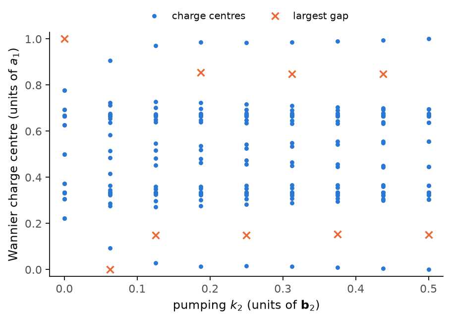
The figure shows the 30 centres of the 30 occupied bands at the 9 steps of \(k_2\), and the line of the largest gap as crosses. Most centres stay close to 1/3 and 2/3 of the cell, which are the positions of the two bismuth atoms along \(\mathbf a_1\), so these are the localized states that do not move. At \(k_2 = 0\) and \(k_2 = 1/2\) the centres come in degenerate Kramers pairs. The pair at 0.222 and 0.778 at \(k_2 = 0\) splits, and one partner of each goes to the edge of the cell, which it reaches as the pair at 0 and 1 at \(k_2 = 1/2\), while the other partner joins the centres near 0.3 and 0.7. So the partners switch, and a line at 0.15 is crossed once in half the zone, which is \(\nu = 1\), the same answer as the parities.

The line of the largest gap is not smooth, however. From \(k_2 = 1/8\) on it jumps between 0.15 and 0.85 at every step, so flow.gap_step is 0.305. The reason is the inversion centre, which maps the centres at \(x\) onto \(1 - x\), so the two gaps near 0.15 and 0.85 have the same size and the code can pick either of them at each step. The count of crossings against such a line can be wrong, and refining the mesh does not help, because the two gaps stay equal. So on a crystal with an inversion centre we take the parity answer as the result and the flow as a picture of it, and here the two agree. On a crystal without inversion the flow is the only route, and there you refine nloop and npump until \(\nu\) does not change.

Code of this figure (docs/figures/topology_wannier_flow/)

compute.py

"""The flow of the Wannier charge centres of a Bi(111) bilayer."""
from defuqumat import Calculator
from common import PSEUDO, save

calc = Calculator.from_file("bi-bilayer.in", pseudo_dir=PSEUDO)
flow = calc.get_z2(nloop=16, npump=9)            # Wilson loops, the default
print("z2 =", flow.z2, " gap_step = %.3f" % flow.gap_step, flush=True)

save(pump=flow.pump, centers=flow.centers_fractional,
     gap=flow.gap_center, z2=flow.z2, gap_step=flow.gap_step)

plot.py

"""The Wannier charge centres of the Bi(111) bilayer, over half the zone."""
import numpy as np
import style

d = np.load("data.npz")


def draw():
    fig, ax = style.figure()
    for n in range(d["centers"].shape[1]):
        ax.plot(d["pump"], d["centers"][:, n], "o", ms=3, color=style.color(0),
                label="charge centres" if n == 0 else None)
    gap = (d["gap"] / (2 * np.pi)) % 1.0
    ax.plot(d["pump"], gap, "x", ms=6, mew=1.5, color=style.color(1), label="largest gap")
    ax.set_xlim(-0.02, 0.52)
    ax.set_ylim(-0.03, 1.03)
    ax.set_xlabel(r"pumping $k_2$ (units of $\mathbf{b}_2$)")
    ax.set_ylabel("Wannier charge centre (units of $a_1$)")
    ax.legend(loc="upper center", bbox_to_anchor=(0.5, 1.12), ncol=2)
    return fig


style.main(draw)

Three dimensions

In three dimensions there are four invariants, written \((\nu_0;\nu_1\nu_2\nu_3)\). Each of the six planes \(k_i = 0\) and \(k_i = 1/2\) has a two-dimensional \(\mathbb Z_2\). The strong index \(\nu_0\) is the sum of the two planes of one direction, modulo 2, and it is the same for all three directions. The weak index \(\nu_i\) is the invariant of the plane \(k_i = 1/2\). With the parity route, \(\nu_0\) is the product of the eight \(\delta_i\). A strong topological insulator has \(\nu_0 = 1\) and a surface Dirac cone on every surface, which ARPES sees. We compute it with calc.get_z2_3d(), here on the same bilayer, which in the code is a crystal of bilayers stacked along \(z\) with vacuum between them:

print(bilayer.get_z2_3d(method="parity"))

(0; 001)

The result is \((0;001)\), which is what a stack of quantum spin Hall layers must give. Along \(\mathbf b_3\) the layers are separated by vacuum, so the bands do not depend on \(k_3\), and the planes \(k_3 = 0\) and \(k_3 = 1/2\) have the same invariant, \(\nu = 1\), which is the value of the previous section. Their sum modulo 2 is \(\nu_0 = 0\), and the plane \(k_3 = 1/2\) gives \(\nu_3 = 1\). The planes \(k_1 = 1/2\) and \(k_2 = 1/2\) contain the direction \(\mathbf b_3\), along which nothing happens, so \(\nu_1 = \nu_2 = 0\). This is what is called a weak topological insulator, and for a real three-dimensional crystal you want \(\nu_0\), which here is zero because the layers do not talk to each other.

Limits

A collinear run with nspin = 2 has two Hamiltonians, one for each spin. So you give the spin channel, spin=0 or spin=1, to get_berry_curvature and get_chern, and without it you get an error. The number of occupied bands is the number of electrons in that channel. Without spin-orbit coupling the Chern number of one channel is always zero, by time reversal inside the channel, while the curvature at each k-point is not. The kubo method and the orbital magnetization still give an error at nspin = 2.

Every invariant gives an error if the occupied bands come closer than 1e-4 Ry to the band above them at any point of the mesh, because the invariant of a set of bands that touches the next one is not defined. If the number of electrons does not fill a whole number of bands, you give nocc, and otherwise this gives an error.

The \(\mathbb Z_2\) invariant gives an error without noncolin = .true., and you also need lspinorb = .true. and a fully relativistic pseudopotential. Without spin-orbit coupling the bands are spin degenerate, the two copies wind in opposite ways, and \(\nu\) is zero for a reason that has nothing to do with the band structure. method="parity" gives an error if the crystal has no inversion centre, and then you use method="wilson". A crystal without magnetization has \(C = 0\) by time reversal.

method="kubo" is for the map, and method="fhs" is for the integer, because the Kubo sum diverges where two bands meet and its sum over the mesh is never an exact integer. The Kubo sum over the empty bands stops at nbnd, and nbnd no larger than nocc gives an error, since the sum is then empty. .truncation says what the highest empty band was worth. Where symmetry makes the curvature zero, this ratio is noise, so you read .truncation_abs there.

The curvature of one band, curvature_by_band, is defined only for a band that is not degenerate. Inside a degenerate level only the sum over its bands has a meaning, and the total curvature always has one. Two bands closer than degeneracy_tol count as one level. If you do not give it, we take the larger of 1e-6 Ry and the split the eigensolver leaves between two exactly degenerate bands, and at the default conv_thr this is 1e-6 Ry. If you give a value below the one we would take, we warn you and still use your value.

With a PAW dataset the invariants need the converged becsum beside the density, because it cannot be rebuilt from the density. The Calculator methods pass it for you.

With a potential-only meta-GGA (tb09 or bj06) the invariants need the converged tau beside the density, for the same reason. The Calculator methods pass it for you. The Berry-phase polarization and the orbital magnetization still give an error with these functionals.

The notebook for this page is 10, the topological invariants.