Diffraction and nesting

In this page we compute two quantities in reciprocal space from a converged ground state. The first is the structure factor, the Fourier coefficient of the density on a reciprocal lattice vector, which is what X-ray and neutron diffraction measure. The second is the nesting function of the Fermi surface, which tells us at which wavevector a metal is closest to an instability.

Structure factors

A diffraction experiment does not measure the density itself. It measures one Fourier coefficient of it per reflection, and this coefficient is the structure factor:

\[ F(\mathbf H) = \int_\Omega \rho(\mathbf r)\, e^{i\mathbf H\cdot\mathbf r}\, d^3r, \qquad F_j(\mathbf H) = \int_\Omega m_j(\mathbf r)\, e^{i\mathbf H\cdot\mathbf r}\, d^3r , \]

for every reciprocal lattice vector \(\mathbf H\) with \(|\mathbf H|\) below a cutoff hmax. X-rays scatter on the charge, so they see \(F\), and neutrons scatter on the magnetization, so they see \(F_j\). \(F(0)\) is the number of electrons in the cell and \(F_j(0)\) is the magnetic moment of the cell, in Bohr magnetons.

A pseudopotential calculation has only the valence electrons, and the core electrons give most of the X-ray scattering of an allowed reflection. So these are valence structure factors, and an allowed reflection is not the measured one. There is one class of reflections where the core does not matter. In a forbidden reflection the spherical part of every atom cancels by symmetry, so what is left is the bonding charge between the atoms, and this is what a pseudopotential describes well. Here we take silicon. We compute it with calc.get_structure_factors():

from defuqumat import Calculator

silicon = Calculator.from_file("docs/figures/scattering_forbidden_reflection/si.in",
                               pseudo_dir="tests/data/pseudo")
factors = silicon.get_structure_factors(hmax=5.0)

print(factors.table(limit=10))

     h     k     l  mult         |H|          Re F          Im F           |F|
------------------------------------------------------------------------------
     0     0     0     1    0.000000      8.000000      0.000000      8.000000
     1    -1    -1     4    1.066941      1.237103     -1.237103      1.749529
     1     1    -1     4    1.066941      1.237103      1.237103      1.749529
     0     0    -2     6    1.231997     -0.000000     -0.000000      0.000000
     2     0    -2    12    1.742307     -0.080712     -0.000000      0.080712
     1    -1    -3    12    2.043036     -0.250196     -0.250196      0.353830
     1     1    -3    12    2.043036     -0.250196      0.250196      0.353830
     2    -2    -2     4    2.133882      0.000000     -0.347404      0.347404
     2     2    -2     4    2.133882      0.000000      0.347404      0.347404
     0     0    -4     6    2.463994     -0.391422     -0.000000      0.391422

Each line is one reflection, with its index \((hkl)\) on the conventional cubic axes, the number of equivalent reflections in its star, \(|\mathbf H|\) in 1/bohr and the complex \(F\) in electrons. The first line is \(F(000) = 8\), the eight valence electrons of the two silicon atoms. The (111), the (311) and the (222) take two rows each, with the same \(|F|\) and opposite imaginary parts, because the code collapses only the members of a star that have the same phase, and in diamond the two halves of these stars differ by a fractional translation. Let us now look at four reflections by their index:

for hkl in [(1, -1, -1), (0, 0, -2), (2, -2, -2), (2, 0, -4)]:
    print(f"{hkl}   |F| = {abs(factors.of(hkl)):.6f}")

(1, -1, -1)   |F| = 1.749529
(0, 0, -2)   |F| = 0.000000
(2, -2, -2)   |F| = 0.347404
(2, 0, -4)   |F| = 0.000000

The (111) reflection is allowed and large, 1.749529 electrons, but most of its measured value comes from the core, so this number is not the measured one. The (200) and the (420) are zero for a different reason. The space group of diamond has a glide plane, and this makes every \((hk0)\) reflection with \(h+k\) not a multiple of 4 exactly zero, whatever the density is inside the cell. The (222) is the interesting one. The space group allows it, and it is zero only if each atom has a spherical charge, because then the two atoms of the cell give equal and opposite amplitudes. So its value, 0.347404 electrons against the 8 of the cell, is a direct measure of the bond charge between the atoms, the part of the density that is not spherical around any atom. This is why the (222) reflection of silicon is measured with X-rays, and it is the reflection where a valence calculation can be compared with experiment.

The keywords of get_structure_factors are:

• hmax: the cutoff on \(|\mathbf H|\), in 1/bohr. If you do not give it, the code takes 6. It cannot be larger than \(\sqrt{\texttt{ecutrho}}\).
• window: an energy window (lo, hi) in Ry, in the same absolute energies as the eigenvalues. The code then builds the density only from the states in the window, so the structure factor becomes a probe of one group of bonding states.
• transform: "conventional" (the default) labels the reflections on the conventional cubic axes of a cubic crystal, and None keeps the indices on the primitive reciprocal vectors. You can also give a 3x3 matrix.
• reduce: if True (the default), the code keeps one reflection of each star, with its multiplicity. False keeps every member.
• core: True adds the partial core charge of a dataset with a nonlinear core correction. This charge is smoothed inside the core, so it moves the small \(|\mathbf H|\) reflections towards the all-electron value but does not reach it.

The result has charge, the complex \(F\) in electrons, and magnetization, the complex \(F_j\) in Bohr magnetons with one column per component (or None for a non-magnetic run). vectors.indices are the \((hkl)\) of the table, vectors.miller the same on the primitive reciprocal vectors, vectors.length is \(|\mathbf H|\) and vectors.multiplicity the size of each star. of(hkl) gives one reflection by the index the table prints, and table() prints the table.

What do neutrons see that X-rays do not? In an antiferromagnet the two sublattices are the same atom with opposite moments, so the charge repeats with half the period of the magnetization. The reflections then split into two sets, one for each probe. Here we take the simplest case, a chain of hydrogen atoms with two atoms per cell and opposite moments. We keep the indices on the primitive vectors and every member of each star:

import numpy as np

chain = Calculator.from_file("docs/figures/scattering_forbidden_reflection/h-afm.in",
                             pseudo_dir="tests/data/pseudo")
afm = chain.get_structure_factors(hmax=2.0, transform=None, reduce=False)

print(f"{'l':>3}{'X-ray |F|':>12}{'neutron |F|':>14}")
for row, (h, k, l) in enumerate(np.asarray(afm.vectors.miller)):
    if h == 0 and k == 0 and l >= 0:
        print(f"{l:>3}{abs(afm.charge[row]):>12.6f}{abs(afm.magnetization[row, 0]):>14.6f}")

  l   X-ray |F|   neutron |F|
  0    2.000000      0.000006
  1    0.000001      1.228710
  2    0.859082      0.000003
  3    0.000000      0.387127

The even reflections, \(l = 0\) and 2, have charge (2.000000 and 0.859082 electrons) and no magnetization, and the odd reflections, \(l = 1\) and 3, have magnetization (1.228710 and 0.387127 \(\mu_B\)) and no charge. So the chain scatters neutrons exactly on the reflections where it does not scatter X-rays. These odd reflections are the superlattice reflections of the antiferromagnet, and seeing them with neutrons is how antiferromagnetic order is found. The magnetization at \(l = 0\) is the total moment of the cell, which is zero for an antiferromagnet. The zeros are zero by symmetry, since shifting the chain by one atom and flipping every spin leaves it unchanged. In the table they are at most \(6\times10^{-6}\), which is the convergence of this SCF, because this input runs with nosym and nothing imposes the symmetry.

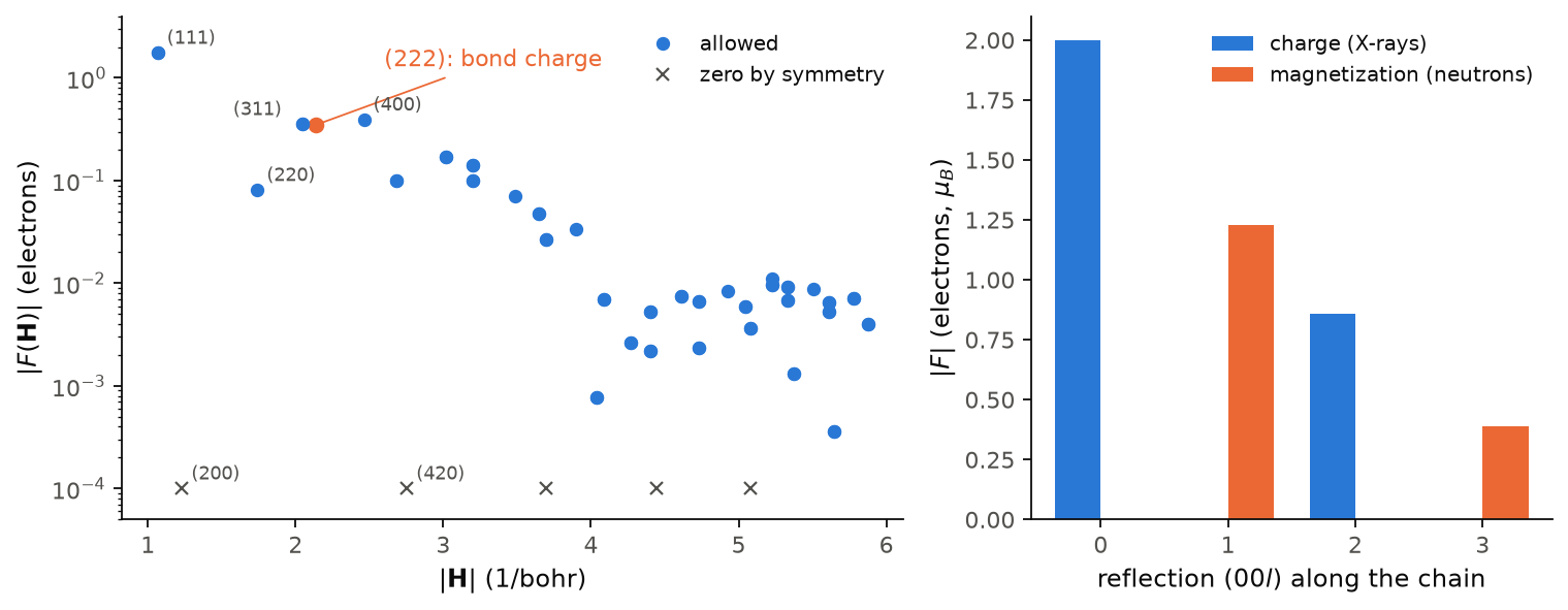
On the left we see the reflections of silicon up to \(|\mathbf H| = 6\) 1/bohr (the figure takes hmax=6.0), on a logarithmic scale. The allowed reflections fall from 1.75 electrons at (111) to about \(10^{-2}\) and below past 4 1/bohr, because the valence density is smooth. The five reflections that the glide plane forbids, (200), (420), (600), (640) and (820), are at most \(4\times10^{-17}\), and we draw them at \(10^{-4}\) with a cross. The (222) reflection, in orange, is 0.347 electrons, about the same as the valence part of its allowed neighbours (311) and (400), so the bond charge is not a small part of the valence density. Next to a measured allowed reflection, which includes the core, the (222) is still a weak reflection. Note that the (222) is the difference of two nearly equal atomic contributions, so it converges more slowly than the total energy. For this reason the input takes a cutoff of 30 Ry and an \(8\times8\times8\) k-mesh, and we did not test its convergence further on this page. On the right we see the hydrogen chain of the snippet above, where charge and magnetization take turns on the reflections along the chain.

Code of this figure (docs/figures/scattering_forbidden_reflection/)

compute.py

"""The X-ray structure factors of silicon, and X-ray against neutron on an antiferromagnet."""
import numpy as np
from defuqumat import Calculator
from common import PSEUDO, save

silicon = Calculator.from_file("si.in", pseudo_dir=PSEUDO)
si = silicon.get_structure_factors(hmax=6.0)

# two hydrogen atoms with opposite moments: keep the primitive (0 0 l) along the chain
chain = Calculator.from_file("h-afm.in", pseudo_dir=PSEUDO)
afm = chain.get_structure_factors(hmax=2.0, transform=None, reduce=False)
miller = np.asarray(afm.vectors.miller)
rows = [r for r in range(len(afm)) if miller[r, 0] == 0 and miller[r, 1] == 0 and miller[r, 2] >= 0]
rows = sorted(rows, key=lambda r: miller[r, 2])

save(hkl=np.asarray(si.vectors.indices), length=np.asarray(si.vectors.length),
     F=np.abs(si.charge), multiplicity=np.asarray(si.vectors.multiplicity),
     l=miller[rows, 2], xray=np.abs(afm.charge[rows]),
     neutron=np.abs(afm.magnetization[rows, 0]))

plot.py

"""Silicon's structure factors against |H|, and X-ray against neutron on a chain."""
import numpy as np
import style

d = np.load("data.npz")
FLOOR = 1e-4          # reflections that are zero by symmetry are drawn here


def label(hkl):
    return "(" + "".join(str(abs(int(v))) for v in sorted(np.abs(hkl), reverse=True)) + ")"


def draw():
    fig, (a, b) = style.figure(2, gridspec_kw={"width_ratios": [3, 2]})
    zero = d["F"] < 1e-8
    bond = np.array([label(h) == "(222)" for h in d["hkl"]])
    keep = (d["length"] > 0) & ~bond
    a.semilogy(d["length"][keep & ~zero], d["F"][keep & ~zero], "o", color=style.color(0),
               label="allowed")
    a.semilogy(d["length"][keep & zero], np.full((keep & zero).sum(), FLOOR), "x",
               color=style.ink2(), label="zero by symmetry")
    drawn = set()
    for i in np.flatnonzero(keep | bond):
        name = label(d["hkl"][i])
        if name in drawn:
            continue
        drawn.add(name)
        if name in ("(111)", "(220)", "(311)", "(400)", "(200)", "(420)"):
            y = d["F"][i] if not zero[i] else FLOOR
            dx = -30 if name == "(311)" else 4
            a.annotate(name, (d["length"][i], y), xytext=(dx, 4), textcoords="offset points",
                       color=style.ink2(), fontsize=8)
        if name == "(222)":
            a.semilogy(d["length"][i], d["F"][i], "o", ms=6, color=style.color(1), zorder=1)
            a.annotate("(222): bond charge", (d["length"][i], d["F"][i]),
                       xytext=(2.6, 1.3), color=style.color(1),
                       arrowprops=dict(arrowstyle="-", color=style.color(1), lw=0.8))
    a.set_xlabel(r"$|\mathbf{H}|$ (1/bohr)")
    a.set_ylabel(r"$|F(\mathbf{H})|$ (electrons)")
    a.set_ylim(5e-5, 4.0)
    a.legend(loc="upper right")

    w = 0.36
    b.bar(d["l"] - w / 2, d["xray"], w, color=style.color(0), label="charge (X-rays)")
    b.bar(d["l"] + w / 2, d["neutron"], w, color=style.color(1), label=r"magnetization (neutrons)")
    b.set_xticks(d["l"])
    b.set_xlabel(r"reflection $(00l)$ along the chain")
    b.set_ylabel(r"$|F|$ (electrons, $\mu_B$)")
    b.legend(loc="upper right")
    fig.tight_layout()
    return fig


style.main(draw)

Fermi-surface nesting

A metal can lower its energy by opening a gap on its own Fermi surface. This costs little where one piece of the Fermi surface, shifted by a wavevector \(\mathbf q\), falls on another piece. The nesting function counts how much of the Fermi surface does this:

\[ N(\mathbf q) = \frac{1}{N_k}\sum_{\mathbf k} g(\mathbf k)\, g(\mathbf k + \mathbf q), \qquad g(\mathbf k) = g_s \sum_{n} \delta(\varepsilon_{n\mathbf k} - E_F). \]

Here \(g(\mathbf k)\) is the density of states at one k-point, so it is a picture of the Fermi surface on the k-mesh, and \(g_s\) is the spin degeneracy. Where \(N(\mathbf q)\) is large, a perturbation with wavevector \(\mathbf q\) connects many occupied states to many empty states at almost no energy cost. This is where a phonon softens (a Kohn anomaly, seen by inelastic X-ray or neutron scattering), a charge-density wave opens a gap, or a spin spiral chooses its pitch. Note that \(N(\mathbf q)\) is only the geometry of the instability. It knows nothing about how strong the coupling is, so a peak says where to look and not whether the instability happens.

Two exact properties help to read it. The mean of \(N(\mathbf q)\) over all \(\mathbf q\) of the grid is \(D(E_F)^2\), the square of the density of states at the Fermi level. And \(N(0) \ge N(\mathbf q)\) for every \(\mathbf q\), by the Cauchy-Schwarz inequality, so \(\mathbf q = 0\) is always the maximum and says nothing about the crystal. What matters is how close another wavevector comes to \(N(0)\).

Here we take a chain of hydrogen atoms, one atom every 5 bohr, without magnetism. One electron per cell in a band that holds two is half filling, so \(k_F = \pi/2c\) and the Fermi surface is the two points \(\pm k_F\). The wavevector \(2k_F = \pi/c\) takes one point to the other, and in crystal coordinates this is \(q_3 = 1/2\). We compute it with calc.get_nesting():

hydrogen = Calculator.from_file("docs/figures/scattering_nesting/h-chain.in",
                                pseudo_dir="tests/data/pseudo")
nest = hydrogen.get_nesting(grid=(1, 1, 60))

where, peak = nest.peak()
print("peak at q =", where)
print(f"N(q*)/N(0) = {peak / nest.nesting[0]:.4f}")
print(f"D(E_F) = {nest.fermi_dos:.3f} states/Ry")
print(f"mean of N(q) / D(E_F)^2 = {nest.nesting.mean() / nest.fermi_dos**2:.6f}")

peak at q = [0.  0.  0.5]
N(q*)/N(0) = 0.9980
D(E_F) = 7.994 states/Ry
mean of N(q) / D(E_F)^2 = 1.000000

The peak is at \(q_3 = 0.5\), which is \(2k_F\), as we expected from the half filling, and it reaches 99.8% of \(N(0)\), so almost every point of the Fermi surface is nested. The mean of \(N(\mathbf q)\) is \(D(E_F)^2\) to six digits, which is the sum rule above. A peak at \(2k_F\) means that, if the chain is unstable, the modulation has period \(2c\), which doubles the cell. In one dimension at half filling this happens for any coupling. If the lattice takes this modulation, the atoms dimerize, which is the Peierls instability. If the spins take it, the chain orders antiferromagnetically, which is the chain of the previous section. You can test the prediction with a calculation that knows nothing about the Fermi surface, a spin spiral of the same chain relaxed in its wavevector, as in Spin spirals.

The nesting function is a non-self-consistent run. We keep the density of the SCF and compute the bands again on the k-mesh grid, and \(g(\mathbf k)\) is a delta function on the Fermi surface, so this mesh is the convergence parameter of the whole quantity. A mesh that is too coarse does not give a noisy peak. It gives a smooth peak in the wrong place, or no peak at all. The keywords of get_nesting are:

• grid: the Monkhorst-Pack mesh of the Fermi surface. If you do not give it, the code uses the mesh of the SCF, which is rarely enough. An input with an explicit list of k-points has no mesh, so there you must give grid. The q-points are the differences of these k-points, so they lie on an unshifted mesh of the same size, whatever the shift of the k-mesh.
• degauss: the width of the delta function, in Ry. If you do not give it, the code uses the degauss of the SCF.
• smearing: the shape of the delta function. If you do not give it, the code uses a Gaussian, even when the SCF used Methfessel-Paxton or cold smearing.
• nbnd: the number of bands.
• fermi_energy: the Fermi level, in Ry. If you do not give it, the code finds the Fermi level again on the dense mesh.

The result has nesting, \(N(\mathbf q)\) in (states/Ry/cell)\(^2\), and qpoints, the q-points in crystal coordinates. ratio is \(N(\mathbf q)/D(E_F)^2\), which is 1 on average, and fermi_dos is \(D(E_F)\). peak() gives the position and the value of the largest \(N(\mathbf q)\) away from \(\mathbf q = 0\), along(i) gives \(N\) along the crystal axis \(i\) for a line plot, and as_grid() gives \(N(\mathbf q)\) as an array of the shape of the mesh, for a map.

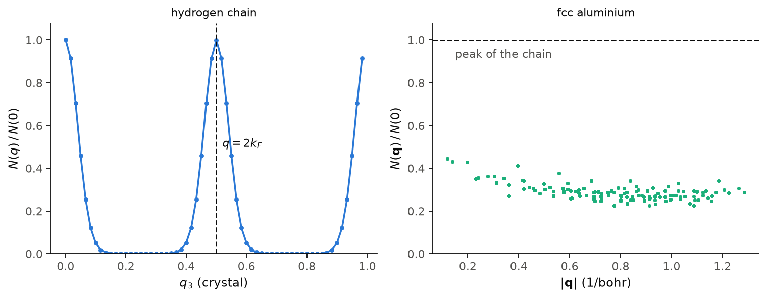
On the left we see \(N(q)/N(0)\) of the hydrogen chain on the 60 q-points of the chain. It has two peaks, at \(q_3 = 0\) and at \(q_3 = 0.5\), of the same height, and it is zero between them. The width of the peaks, about \(\pm0.05\) in \(q_3\) at half height, comes from the Gaussian width degauss = 0.02 Ry of the delta functions. On the right we see fcc aluminium on a \(12\times12\times12\) mesh, with the default Gaussian of the width degauss = 0.05 Ry of its input. All 1727 points away from \(\mathbf q = 0\) lie between 0.23 and 0.45 of \(N(0)\), and the largest one, 0.445, is at the smallest \(|\mathbf q|\) of the mesh, 0.12 1/bohr. So the nesting function of aluminium is a featureless plateau that falls slowly with \(|\mathbf q|\), and nothing rises above it. This is what a nearly spherical Fermi surface gives, since a sphere shifted by \(\mathbf q\) touches itself only on a circle. Aluminium has no charge-density wave and no magnetic order, in agreement with this. We did not converge the aluminium mesh, so the values on the plateau can change on a denser mesh or with a smaller degauss.

Code of this figure (docs/figures/scattering_nesting/)

compute.py

"""The nesting function of a half-filled hydrogen chain and of fcc aluminium."""
import numpy as np
from defuqumat import Calculator
from common import PSEUDO, save

chain = Calculator.from_file("h-chain.in", pseudo_dir=PSEUDO)
nest = chain.get_nesting(grid=(1, 1, 60))
q3, n3 = nest.along(2)
where, peak = nest.peak()

aluminium = Calculator.from_file("al.in", pseudo_dir=PSEUDO)
metal = aluminium.get_nesting(grid=(12, 12, 12))
cell = aluminium.system.cell
q = metal.qpoints - np.rint(metal.qpoints)          # into the first zone
length = np.linalg.norm(cell.k_to_cartesian(q), axis=1) * cell.tpiba
al_where, al_peak = metal.peak()

save(q3=q3, chain=n3 / nest.nesting[0], chain_peak=where, chain_ratio=peak / nest.nesting[0],
     chain_dos=nest.fermi_dos, q=length, metal=metal.nesting / metal.nesting[0],
     metal_peak=al_where, metal_ratio=al_peak / metal.nesting[0], metal_dos=metal.fermi_dos)

plot.py

"""N(q) along the hydrogen chain, and N(q) of aluminium against |q|."""
import numpy as np
import style

d = np.load("data.npz")


def draw():
    fig, (a, b) = style.figure(2)
    a.plot(d["q3"], d["chain"], "o-", ms=3, color=style.color(0))
    a.axvline(0.5, **style.reference())
    a.text(0.52, 0.5, r"$q = 2k_F$", color=style.ink())
    a.set_xlabel(r"$q_3$ (crystal)")
    a.set_ylabel(r"$N(q)\,/\,N(0)$")
    a.set_ylim(0, 1.08)
    a.set_title("hydrogen chain", color=style.ink(), fontsize=10)

    b.plot(d["q"][1:], d["metal"][1:], ".", ms=4, color=style.color(2))
    b.axhline(float(d["chain_ratio"]), **style.reference())
    b.text(0.15, float(d["chain_ratio"]) - 0.08, "peak of the chain", color=style.ink2())
    b.set_xlabel(r"$|\mathbf{q}|$ (1/bohr)")
    b.set_ylabel(r"$N(\mathbf{q})\,/\,N(0)$")
    b.set_ylim(0, 1.08)
    b.set_title("fcc aluminium", color=style.ink(), fontsize=10)
    fig.tight_layout()
    return fig


style.main(draw)

Limits

The structure factors give an error if hmax is larger than \(\sqrt{\texttt{ecutrho}}\). Past the cutoff of the density, the FFT grid still has coefficients, but they are not Fourier components of the density, and they look small and plausible. The structure factors also give an error for an empty or inverted energy window, and for core=True with a dataset that has no nonlinear core correction.

The structure factors are valence structure factors. An allowed reflection is dominated by the core, so it is not the measured value, and only a forbidden reflection compares directly with experiment. The multiplicity of a star applies to the charge. The magnetic members of a star are not equal to each other, so for the magnetization you keep every member with reduce=False.

The nesting function gives an error for a run with fixed occupations (occupations = 'fixed' or 'from_input'), which has no Fermi level, also when it has tot_magnetization. With a smearing, a run with tot_magnetization has one Fermi level for each spin channel, and the delta function of each channel is then at its own level. In that case fermi_energy must be the pair (ef_up, ef_dw) if you give it, and the result has fermi_energy_up and fermi_energy_down. A run with tetrahedra and tot_magnetization still gives an error. It also gives an error for a spin spiral, because the nesting function is a property of the state the spiral grows from. So you compute it on the non-magnetic or collinear state and compare its peak with the wavevector of the relaxed spiral.

The delta function of the nesting function is a Gaussian by default, even when the SCF used Methfessel-Paxton or cold smearing, because those go negative on the wings, so \(g(\mathbf k)\) can be negative and \(N(\mathbf q)\) has no sign. You can still pass smearing= to use the smearing of the run. A run with no degauss, such as one with tetrahedra, gives an error unless you pass degauss yourself.

The notebooks for this page are 37, structure factors and 31, Fermi-surface nesting.