Strain and polarization couplings
In this page we compute how a crystal couples its strain, its polarization and a magnetic field. We start with the piezoelectric tensor, the polarization that a strain creates, and its convergence with the k-mesh. Then we compute the elasto-optic and electrostriction tensors, which say how a strain changes the dielectric response, and finally the magnetoelectric tensor, the polarization that a magnetic field creates.
The piezoelectric tensor
We start with the simplest coupling, which is linear in both the strain and the field. The piezoelectric tensor is the polarization that a strain creates, at zero field:
The first two forms are the same number, because a mixed second derivative of
the energy does not depend on the order, meaning that the polarization a strain
creates is also the stress a field creates. This is what a piezoelectric sensor
reads as a voltage, and what a piezoelectric actuator uses in reverse. A tensor
with three Cartesian labels is zero in every crystal with an inversion centre,
so silicon has none, and AlAs, the same lattice with two different atoms on the
two sublattices, has one. We compute it with calc.get_piezoelectric_tensor():
import numpy as np
from defuqumat import Calculator

alas = Calculator.from_file("docs/figures/piezo_components/alas.in",
                            pseudo_dir="tests/data/pseudo")
piezo = alas.get_piezoelectric_tensor()
print(np.round(piezo.voigt, 4))     # C/m^2, columns xx yy zz yz xz xy
print(f"e14 = {piezo.e14:.4f} C/m^2 from {piezo.nk} k-points, grid {piezo.grid}")
[[-0.      0.      0.     -0.7636  0.     -0.    ]
 [ 0.      0.     -0.      0.     -0.7636  0.    ]
 [-0.     -0.      0.      0.     -0.     -0.7636]]
e14 = -0.7636 C/m^2 from 8 k-points, grid (4, 4, 4)
piezo.voigt is the tensor as a 3 by 6 table, with one row for each direction
of the polarization and one column for each strain, in the Voigt order xx, yy,
zz, yz, xz, xy, and piezo.e is the same tensor with three Cartesian labels, in
\(e/\text{bohr}^2\). We see that only three entries are not zero, \(e_{14} = e_{25}
= e_{36} = -0.7636\) C/m\(^2\), which is what the point group \(\bar 4 3m\) of
zincblende allows, so a cubic crystal of this class has one piezoelectric
constant and piezo.e14 is that number. A shear strain in the \(yz\) plane
creates a polarization along \(x\), and an axial strain creates none. The 64
points of the \(4\times4\times4\) mesh are reduced to 8 by the symmetry of the
crystal, and the code also prints a warning on stderr, because nothing in this
calculation says whether 64 points are enough. We come back to this question
in the next section.
Silicon is the same lattice with an inversion centre, and we check that its tensor is zero:
silicon = Calculator.from_file("docs/figures/piezo_components/si.in",
                               pseudo_dir="tests/data/pseudo")
e_si = silicon.get_piezoelectric_tensor()
print(f"largest component in silicon: {np.abs(e_si.voigt).max():.1e} C/m^2")
largest component in silicon: 7.5e-26 C/m^2
On the reduced mesh the code symmetrizes the tensor with the point group of the
crystal, so here this zero is also imposed by the symmetrization, meaning that
it is a statement about the symmetry and not a test of the calculation. On a
full mesh with nosym nothing imposes it, and there the size of the residue
says how precise the field response is.
The k-mesh of the piezoelectric tensor
How many k-points does the piezoelectric tensor need? The total energy is
variational, so its error is second order in the error of the density, but
\(e_{14}\) is a mixed derivative of that energy, which is a sum over the
Brillouin zone with no such protection, so it needs a denser mesh than the
ground state does. Nothing inside one calculation can see this, so the way we
check it is by running the whole calculation again on a ladder of meshes and
looking at how much the last step moved the tensor. We compute it with
calc.get_piezoelectric_kmesh_ladder():
ladder = alas.get_piezoelectric_kmesh_ladder(meshes=(4, 6, 8), method="zstar_eu")
print(ladder.nk)                    # k-points of each rung, after symmetry
print(np.round(ladder.e14, 4))      # C/m^2
print(f"last step {ladder.drift:.3f}, settled: {ladder.settled}")
(8, 16, 29)
[-0.7636 -0.6874 -0.6729]
last step 0.022, settled: False
Each rung is an unshifted \(n\times n\times n\) mesh with a new ground state and a
new field response, and no rung starts from the one below it, so each number is
a calculation of its own. ladder.steps is the change of the whole tensor
across each step, relative to its largest component, ladder.drift is the last
of them, and ladder.settled says whether it is below 1 per cent. We see that
\(e_{14}\) moves by 11 per cent from \(4^3\) to \(6^3\) and by 2.2 per cent from
\(6^3\) to \(8^3\), so the \(4^3\) mesh of the first section is far from converged
for this quantity, and you should converge the mesh on \(e_{14}\) itself rather
than on the total energy. The option
method="zstar_eu" gives the same tensor by a cheaper route that holds
much less memory, so it is the method to use when you converge the mesh.
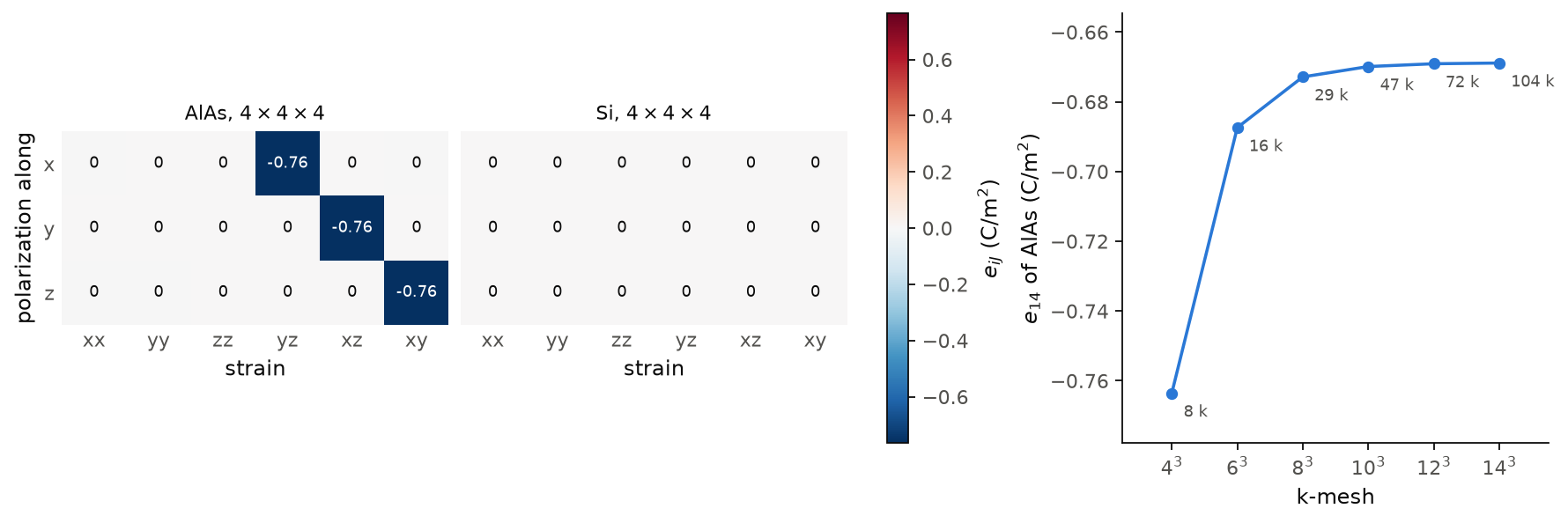
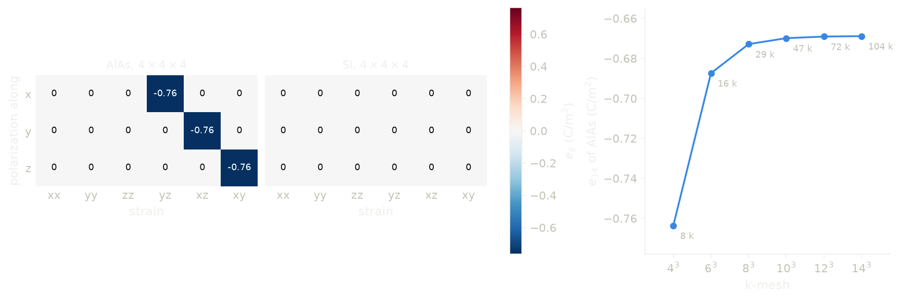
The two tables on the left are the tensors of the first section, AlAs and
silicon on the \(4\times4\times4\) mesh, with the polarization direction in the
rows and the strain in the columns. AlAs has the three equal shear entries
\(e_{14} = e_{25} = e_{36} = -0.76\) C/m\(^2\), and silicon has no entry at all.
The right panel is the ladder continued to \(14\times14\times14\), with the
number of k-points of each rung after symmetry. We see that \(e_{14}\) goes from
\(-0.7636\) at \(4^3\) to \(-0.6699\) at \(10^3\), \(-0.6691\) at \(12^3\) and \(-0.6689\)
C/m\(^2\) at \(14^3\), and the relative steps are 11, 2.2, 0.44, 0.12 and 0.03 per
cent, so they shrink by a factor of four to five each rung. The \(4^3\) value is
14 per cent larger in size than the \(14^3\) one, and we need at least the
\(8\times8\times8\) mesh, 29 points, to be within 1 per cent. The six rungs
took 87 s on one core together. The ladder converges only the k-mesh, and on
this cell, with ecutwfc = 10 Ry, the cutoff changes
\(e_{14}\) by about 1 per cent, so you converge ecutwfc separately. Note that this is the clamped-ion tensor, so
the \(-0.67\) C/m\(^2\) is not yet the value one measures, as we say in the Limits
below.
Code of this figure (docs/figures/piezo_components/)
"""The piezoelectric tensor of AlAs and silicon, and e_14 of AlAs on a ladder of k-meshes."""
import numpy as np
from defuqumat import Calculator
from common import PSEUDO, save

alas = Calculator.from_file("alas.in", pseudo_dir=PSEUDO)
silicon = Calculator.from_file("si.in", pseudo_dir=PSEUDO)
alas_e = alas.get_piezoelectric_tensor(kmesh_warning=False).voigt     # (3, 6), C/m^2
silicon_e = silicon.get_piezoelectric_tensor(kmesh_warning=False).voigt

ladder = alas.get_piezoelectric_kmesh_ladder(meshes=(4, 6, 8, 10, 12, 14), method="zstar_eu",
                                             verbose=True)
save(alas=alas_e, silicon=silicon_e, meshes=np.array(ladder.meshes),
     nk=np.array(ladder.nk), e14=np.array(ladder.e14), steps=np.array(ladder.steps),
     seconds=np.array(ladder.seconds))
"""The piezoelectric tensor of AlAs and silicon, and e_14 of AlAs against the k-mesh."""
import numpy as np
import style

d = np.load("data.npz")
strains = ["xx", "yy", "zz", "yz", "xz", "xy"]


def table(ax, e, title, scale):
    m = ax.imshow(e, cmap="RdBu_r", vmin=-scale, vmax=scale, aspect="equal")
    for i in range(3):
        for j in range(6):
            dark = abs(e[i, j]) > 0.5 * scale
            text = "0" if abs(e[i, j]) < 5e-3 else f"{e[i, j]:.2f}"
            ax.text(j, i, text, ha="center", va="center", fontsize=8,
                    color="white" if dark else "#0b0b0b")
    ax.set_xticks(range(6), strains)
    ax.set_yticks(range(3), ["x", "y", "z"])
    ax.set_xlabel("strain")
    ax.set_title(title, fontsize=10, color=style.ink())
    for side in ("top", "right", "bottom", "left"):
        ax.spines[side].set_visible(False)
    ax.tick_params(length=0)
    return m


def draw():
    fig, (a, b, c) = style.figure(3, gridspec_kw={"width_ratios": [1.0, 1.0, 1.1]},
                                layout="constrained")
    scale = np.abs(d["alas"]).max()
    table(a, d["alas"], "AlAs, $4\\times4\\times4$", scale)
    a.set_ylabel("polarization along")
    m = table(b, d["silicon"], "Si, $4\\times4\\times4$", scale)
    b.set_yticks(range(3), [])
    style.colorbar(fig, m, [a, b], r"$e_{iJ}$ (C/m$^2$)")

    c.plot(d["meshes"], d["e14"], "o-", color=style.color(0))
    for n, nk, e in zip(d["meshes"], d["nk"], d["e14"]):
        c.annotate(f"{nk} k", (n, e), textcoords="offset points", xytext=(6, -12),
                   fontsize=8, color=style.ink2())
    c.set_xticks(d["meshes"], [f"${n}^3$" for n in d["meshes"]])
    c.set_xlabel("k-mesh")
    c.set_ylabel(r"$e_{14}$ of AlAs (C/m$^2$)")
    c.margins(x=0.15, y=0.15)
    return fig


style.main(draw)
Electrostriction and the elasto-optic tensor
We now go one order higher. Every insulator deforms in an electric field, also one with an inversion centre, because the stress is quadratic in the field, \(\sigma_{ij} \propto m_{ijkl}\,\mathcal E_k \mathcal E_l\), and this is electrostriction, which is measured as the strain of a dielectric under a field. The same coupling in reverse is how a strain changes the dielectric response, and the elasto-optic tensor, the change of the inverse dielectric tensor per unit strain, is what Brillouin scattering and acousto-optic modulators measure. Here we write the strain as \(x\):
Here \(\chi\) is the electronic susceptibility and
\(\eta = \chi^{-1}\) its inverse, so all of them come from one quantity,
\(\partial\chi/\partial x\), which is a third derivative of the energy, two
fields and one strain. The code gets it from the first-order wavefunctions of
the field and of the strain alone, by the \(2n+1\) theorem, so no second-order
wavefunction is needed. We compute it with calc.get_electrostriction(), here
for silicon on a \(20\times20\times20\) mesh:
silicon = Calculator.from_file("docs/figures/piezo_components/si-optic.in",
                               pseudo_dir="tests/data/pseudo")
es = silicon.get_electrostriction(elastic=False)
print(f"epsilon = {np.trace(es.epsilon) / 3:.3f}")
p = es.photoelastic_voigt
print(f"p11 = {p[0, 0]:.4f}   p12 = {p[0, 1]:.4f}   p44 = {p[3, 3]:.4f}")
m_h, q_h = es.hydrostatic
print(f"m_h = {m_h:.1f} pN/V^2   q_h = {q_h:.3f} GN m^2/C^2")
epsilon = 12.606
p11 = -0.0957   p12 = 0.0239   p44 = -0.0777
m_h = -33.6 pN/V^2   q_h = -3.186 GN m^2/C^2
es.photoelastic is the elasto-optic tensor \(p_{ijkl}\) with four labels and
es.photoelastic_voigt the same as a 6 by 6 table, so a cubic crystal has the
three numbers \(p_{11}\), \(p_{12}\) and \(p_{44}\). es.m and es.q are the two
electrostriction tensors at fixed strain, in pN/V\(^2\) and GN m\(^2\)/C\(^2\), and
es.hydrostatic gives the combinations \(m_{11} + 2m_{12}\) and
\(q_{11} + 2q_{12}\), which are the ones a hydrostatic strain sees. We pass
elastic=False because the elastic constants need the full k-mesh, and this
input is reduced by symmetry, so without it the call gives an error. Then
es.M and es.Q, the two tensors at fixed stress, are None, because they
need the elastic compliance.
Why such a dense mesh? The elasto-optic tensor is a small change of the
dielectric tensor, and it converges slowly with the k-mesh. The run above takes
109 s on one core with the kernels already compiled, and in separate runs of the same input on smaller meshes, \(p_{11}\)
reads \(-0.0544\), \(-0.0746\), \(-0.0871\), \(-0.0927\), \(-0.0947\) and \(-0.0953\) at
\(6^3\), \(8^3\), \(10^3\), \(12^3\), \(14^3\) and \(16^3\), and \(p_{12}\) reads \(-0.0026\)
at \(6^3\) and \(+0.0085\) at \(8^3\), so on a \(6\times6\times6\) mesh even its sign
is wrong. From \(16^3\) to \(20^3\), \(p_{11}\) still moves by 0.4 per cent and
\(p_{12}\) by 1.7 per cent, so the last digit printed above is not converged. The
dielectric constant moves in the same way, from 15.744 at \(6^3\) to 12.617 at
\(16^3\) and 12.606 at \(20^3\). All these numbers are at ecutwfc = 12 Ry, and
we did not converge the cutoff. As a reference, the measured values for silicon are
\(p_{11} = -0.094\), \(p_{12} = +0.017\) and \(p_{44} = -0.051\). The clamped-ion
\(p_{11}\) and \(p_{12}\) are the whole answer in the diamond structure, while
\(p_{44}\) misses the relaxation of the atoms inside the cell, so it is not yet
a number to compare with the measured one.
The magnetoelectric tensor
We now replace the strain by a magnetic field. The magnetoelectric tensor is the polarization that a magnetic field creates:
It is measured as the charge, or the voltage, that appears on a crystal when a
magnetic field is applied, and it is what a voltage-written magnetic memory
would use in reverse. Time reversal and inversion both change the sign of
\(\alpha\), so it is zero whenever one of the two is a symmetry. AlAs has no
inversion centre, and here a static field in the input breaks time reversal, so
we compute the response to a small further change of that field. The direction
of the field matters. Along a cube axis, for example \(B_z\), the field keeps the
twofold rotation and the fourfold rotoinversion about \(z\), which flip \(P_x\),
\(P_y\) and \(P_z\), so the polarization is zero for every field along \(z\) and the
whole column \(\partial P/\partial B_z\) is zero by symmetry. The response that
zincblende allows is quadratic in the field, \(P_x \propto B_y B_z\), so its
derivative is not zero only when the field has components along more than one
cube axis. Here we put the field along the cube diagonal \([111]\), and for this
the input uses the rhombohedral setting of the same fcc lattice (ibrav = 5),
in which \(z\) is \([111]\). The threefold axis then forces \(P_x = P_y = 0\) and
leaves \(P_z\) free. The field acts on the spin and the polarization is a
property of the charge, so the two are coupled only through spin-orbit
coupling. Without it the tensor is exactly zero, because a uniform field on the
spin then only shifts the bands of the two spins of this insulator rigidly, so
the charge does not change at all. The code computes each column of \(\alpha\)
as a central difference of the Berry-phase polarization between two
self-consistent runs at \(B \pm \delta/2\). We compute it with
calc.get_magnetoelectric_tensor(), with and without spin-orbit coupling:
alas = Calculator.from_file("docs/figures/piezo_components/alas-field.in",
                            pseudo_dir="tests/data/pseudo")
me = alas.get_magnetoelectric_tensor(delta=0.02, directions=(2,),
                                     nppstr=6, transverse=(2, 2))
print(me.alpha[:, 2])               # dP/dB_z, along x, y and z

no_soc = Calculator.from_file("docs/figures/piezo_components/alas-field-nosoc.in",
                              pseudo_dir="tests/data/pseudo")
null = no_soc.get_magnetoelectric_tensor(delta=0.02, directions=(2,),
                                         nppstr=6, transverse=(2, 2))
print(null.alpha[:, 2])             # the same column without spin-orbit coupling
[3.76382078e-10 9.58366487e-11 3.17899747e-06]
[-1.80241501e-10 -4.09963801e-10  1.05013792e-09]
directions=(2,) steps only the \(z\) component of the field, which costs two
self-consistent runs, so only the third column of me.alpha is computed, and
the other two are left at zero. delta is the size of the step, nppstr the
number of k-points along each Berry-phase string and transverse the k-mesh
across the strings. We see that a change of the field along \([111]\) creates a
polarization along \([111]\), \(3.2\times10^{-6}\), while the two components that
the threefold axis forces to zero are \(3.8\times10^{-10}\) and
\(9.6\times10^{-11}\). This is the precision of the two self-consistent runs,
because the k-mesh and the Berry-phase strings keep the threefold symmetry, so
the three string directions are images of one another. Without spin-orbit
coupling the largest entry is \(1.1\times10^{-9}\), the same floor measured a
second way, so the allowed response is about 3000 times above the precision of
the calculation and it comes from spin-orbit coupling. The tensor is in
\(e/\text{bohr}^2\) per unit of the internal field of the code, so its absolute
size is not yet a number to compare with experiment. The \(2\times2\times2\)
ground-state mesh and the 2 by 2 mesh across the strings are also small, and we
did not converge them, so the value \(3.2\times10^{-6}\) is not converged either.
The two runs together took 123 s on one core.
Limits
The piezoelectric tensor is clamped-ion: the atoms move with the strain and
do not relax. The internal-strain part, which makes the constant
comparable with experiment, is not computed, and in zincblende crystals it
almost cancels the clamped-ion part. A polar crystal, one whose crystal
class leaves a direction invariant, gives an error, because there the
measured tensor differs from the derivative by terms built from the
spontaneous polarization. A PAW dataset gives an error, while
norm-conserving and ultrasoft datasets work on any k-mesh. The tensor
needs an insulator with nspin = 1, and it gives an error for a metal, a
spin spiral, a magnetic field, and a shifted k-mesh with nosym. If the
field response under the tensor does not converge, the code gives an error
instead of using it. The code warns that the k-mesh may be
too coarse, because nothing inside one calculation can see it, and
kmesh_warning=False silences the warning once you have converged the
mesh with the ladder.
The electrostriction and elasto-optic tensors are clamped-ion too, and they
need an insulator with nspin = 1. In the diamond structure a tetragonal
strain moves no atom inside the cell, so \(p_{11}\) and \(p_{12}\) of silicon
are complete, while \(p_{44}\) misses the term from the internal displacement
of the atoms. They work on norm-conserving, ultrasoft
and PAW datasets, but the elastic constants are norm-conserving only, so
for an ultrasoft or PAW dataset you pass elastic=False, and then M and
Q are None, because they need the elastic compliance. The elastic
constants also need the full k-mesh (nosym), so on a symmetry-reduced
mesh you pass elastic=False as well. The elasto-optic tensor and the
electrostriction tensors m and q work on the symmetry-reduced mesh,
and only M and Q are left out there. If one of the two linear
responses under the calculation does not converge, the code gives an error
instead of using it.
The magnetoelectric tensor gives an error if a ground state does not
converge. On the AlAs cell of this page, only the column along the
starting magnetization converges, because a field with a transverse
component has to rotate the moment, and this is slow, so you start the
magnetization along the column you want. The tensor needs a noncollinear
run that carries a magnetization vector (nspin_mag = 4). Any other run
gives an error, because the field then acts on nothing and every
polarization is the same. This includes every collinear run, with
nspin = 1 or nspin = 2, and a noncollinear run with no
starting_magnetization and no applied field. In the last case you set
one of the two. A field step
that moves the Berry phase by more than a quarter of its quantum gives an
error, and so does everything the Berry-phase polarization refuses. The
field acts only on the spin, so the orbital part of the coupling is not
included, and the atoms are clamped. The field is in the internal unit of
the code, so the absolute size of the tensor is not yet a number to
compare with experiment or with another code.
The notebooks for this page are 28, piezoelectricity, 21, electrostriction and 35, the magnetoelectric effect.