Starting from an all-electron ground state

In this page we compute a ground state that starts from the converged density of Elk, an all-electron LAPW code, and we compare the two densities point by point. We take simple cubic hydrogen at \(a = 3.0\) bohr, which has no core electrons, so the all-electron density and the valence density count the same single electron.

Reading the all-electron density

An all-electron code and a pseudopotential code do not converge to the same density. The all-electron density has every electron of the atom and the cusp at the nucleus, while the pseudopotential density is a smooth valence density, which is built to agree with the true one only outside a cutoff radius around each atom. Elk stores its density in two parts. Inside a sphere of radius \(r_a\) around each atom, the muffin-tin sphere, it is an expansion in real spherical harmonics on a radial mesh, and outside all spheres it is a Fourier series:

\[ \rho(\mathbf r) = \begin{cases} \sum_{lm} f_{lm}(r)\,R_{lm}(\hat{\mathbf r}), & |\mathbf r - \mathbf R_a| < r_a,\\[4pt] \sum_{\mathbf G} \tilde\rho(\mathbf G)\, e^{i\mathbf G\cdot\mathbf r}, & \text{otherwise.} \end{cases} \]

To put this density on our grid, the code asks for each grid point which region it is in, and then it interpolates the radial functions or sums the Fourier series. The points inside a sphere are evaluated one by one, so the cusp is not cut by a Fourier truncation on the grid. The run itself cuts it at its first iteration, as we will see in the next section.

We compute it with calc.get_elk_seed():

from defuqumat import Calculator

calc = Calculator.from_file("docs/figures/elk-seed_hydrogen/h.in",
                            pseudo_dir="tests/data/pseudo")
report = []
seed = calc.get_elk_seed("docs/figures/elk-seed_hydrogen/elk", report=report)
print(seed.shape)
print(f"charge before scaling   {report[0].integral:.6f}")
print(f"charge in the sphere    {report[0].muffin_tin:.6f}")

(1, 15, 15, 15)
charge before scaling   1.000298
charge in the sphere    0.612576

The argument of get_elk_seed is the folder of an Elk run, with STATE.OUT and GEOMETRY.OUT side by side. STATE.OUT has the density but not the lattice vectors or the atomic positions, so the code reads them from GEOMETRY.OUT, which is also the only file written in the frame Elk really used. The elk.in that made this run is in the same folder. The seed has the shape (spin, grid), here one channel on the \(15^3\) grid of the run. The Elk density integrates to 1.000298 electrons on our grid, and the code scales it to the valence charge of the run, here exactly 1, unless you pass renormalise=False. Of this one electron, 0.612576 is inside the muffin-tin sphere of the hydrogen atom. The list you pass as report receives these numbers, and you can leave it out.

Starting the SCF from it

We now give the Elk density to get_scf as the starting density, and we compare with a normal run, which starts from a sum of atomic charges:

seeded = calc.get_scf(starting_density=seed)
plain = Calculator.from_file("docs/figures/elk-seed_hydrogen/h.in",
                             pseudo_dir="tests/data/pseudo").get_scf()
print(f"from the Elk density   {seeded.total_energy:.12f} Ry  {seeded.iterations} iterations")
print(f"from atomic charges    {plain.total_energy:.12f} Ry  {plain.iterations} iterations")

from the Elk density   -1.080181442650 Ry  4 iterations
from atomic charges    -1.080181442649 Ry  4 iterations

Both runs take four iterations and end at the same total energy, to \(10^{-12}\) Ry, so the SCF of the pseudopotential code still decides the answer and the seed only decides where it starts. Here the seed saves no iterations at all. For a hydrogen atom the sum of atomic charges is already close to the answer, and the part where the Elk density is different from it is the cusp, which is in the region where the pseudopotential density is built not to follow it. So what get_elk_seed gives you is the bridge itself: an all-electron ground state, computed in a different basis, on the grid of this code, where you can compare it with the pseudopotential density point by point.

The run also prints a warning that 2 per cent of the starting density is not symmetric. This is the part of the cusp at wave vectors beyond the cutoff of the run, which the first iteration drops. The seed itself has the full symmetry of the cube, so you can ignore the warning here.

Where the two densities differ

We now compare the two densities at the atom:

print(f"at the atom, Elk        {float(seed[0, 0, 0, 0]):.4f} e/bohr^3")
print(f"at the atom, converged  {float(seeded.density[0, 0, 0, 0]):.4f} e/bohr^3")

at the atom, Elk        0.2858 e/bohr^3
at the atom, converged  0.1762 e/bohr^3

At the nucleus the converged pseudopotential density is 38 per cent lower than the all-electron one, which is the cusp that the pseudopotential removes on purpose.

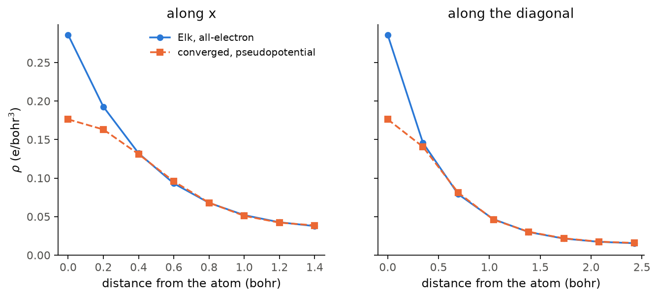
The figure shows the two densities on the grid points of the run, from the atom to the middle of the cell, along \(x\) (left) and along the diagonal of the cube (right). We see that the all-electron density falls steeply from the atom while the pseudopotential density is flat there. At 0.2 bohr along \(x\) they are still 15 per cent apart, and from 0.4 bohr outwards they agree to within 3 per cent on both lines, the largest difference being 2.8 per cent at 0.6 bohr along \(x\). Both runs use a \(4\times4\times4\) k-mesh, which is not converged for this metal, and the Elk run uses its default smearing, LDA parametrization and basis, not the Gaussian smearing of 0.02 Ry and the PZ LDA of h.in. So this 3 per cent is an upper estimate, which includes the error of the pseudopotential but also these differences in the settings. Note that the grid has a spacing of 0.2 bohr along \(x\) and 0.35 bohr along the diagonal, so the cusp is seen at one grid point only, and the lines between the points are only a guide to the eye.

Code of this figure (docs/figures/elk-seed_hydrogen/)

compute.py

"""Hydrogen started from the Elk density, and from atomic charges."""
import numpy as np
from defuqumat import Calculator
from common import PSEUDO, save

calc = Calculator.from_file("h.in", pseudo_dir=PSEUDO)
seed = calc.get_elk_seed("elk")
seeded = calc.get_scf(starting_density=seed)
plain = Calculator.from_file("h.in", pseudo_dir=PSEUDO).get_scf()

# the grid points on the line from the atom along x, and along the diagonal
n = seed.shape[1]
i = np.arange(n)
save(x=i * 3.0 / n, d=i * 3.0 * np.sqrt(3.0) / n,
     seed_x=seed[0, i, 0, 0], scf_x=seeded.density[0, i, 0, 0],
     seed_d=seed[0, i, i, i], scf_d=seeded.density[0, i, i, i],
     energies=[seeded.total_energy, plain.total_energy],
     iterations=[seeded.iterations, plain.iterations])

plot.py

"""The Elk density of hydrogen and the converged pseudo density, through the atom."""
import numpy as np
import style

d = np.load("data.npz")


def draw():
    fig, (a, b) = style.figure(2, sharey=True)
    for ax, key, title in [(a, "x", "along x"), (b, "d", "along the diagonal")]:
        half = d[key] <= d[key].max() / 2 + 1e-9
        r = d[key][half]
        ax.plot(r, d["seed_" + key][half], "o-", color=style.color(0),
                label="Elk, all-electron")
        ax.plot(r, d["scf_" + key][half], "s--", color=style.color(1),
                label="converged, pseudopotential")
        ax.set_xlabel("distance from the atom (bohr)")
        ax.set_title(title, color=style.ink())
        ax.set_xlim(-0.04 * r.max(), 1.04 * r.max())
    a.set_ylabel(r"$\rho$ (e/bohr$^3$)")
    a.set_ylim(0.0, None)
    a.legend()
    return fig


style.main(draw)

Limits

The Elk state must be for the same cell as the run, because a density cannot be moved from one lattice to another. The folder must contain GEOMETRY.OUT from the same Elk run as STATE.OUT. A folder without GEOMETRY.OUT gives an error. A GEOMETRY.OUT with a different number of species, or a different number of atoms in a species, also gives an error. We do not check the atomic positions against STATE.OUT, so you must make sure that both files come from the same run. A STATE.OUT written by Elk older than version 2.0.0 gives an error.

A collinear spin-polarized Elk state can start a run with nspin=2. The code moves the charge and the magnetization of Elk to the grid. Both are scaled by the same factor, so the polarization at each point is the one of Elk. A noncollinear Elk state gives an error. This includes a spin spiral, because STATE.OUT does not say that the run was a spiral. An Elk state with a fixed spin moment also gives an error. A spin-polarized Elk state with an nspin=1 run gives an error, because the moment would be lost. An unpolarized Elk state with an nspin=2 run gives an error, because the seed would have no moment. A noncollinear run gives an error with any Elk state. A DFT+U state works as a seed. STATE.OUT does not contain the occupation matrix of Elk, so only the density is used, and the code gives a warning. The Hubbard occupations then start from starting_ns of the run, as in a normal DFT+U run. A spin-polarized DFT+U state gives an error, because we have not checked the two together. A state with fixed tensor moments gives an error, because the code does not have this constraint.

An element with core electrons gives an error. The muffin-tin density of Elk contains the core states, and nothing in STATE.OUT separates them from the valence charge. So when the Elk density integrates to a charge that is further from the valence charge of the run than half of it (or than 0.5 electrons, if that is larger), the code gives an error and does not scale it. Hydrogen, with no core, is the case this is made for.

The Elk density can only be a starting density. You cannot use it as a fixed density with no SCF on top, because the two converged densities are different functions near every nucleus.

The notebook for this page is 42, starting from an all-electron ground state.