Density of states

In this page we compute the density of states, the number of states per unit energy, and then its projection on the atomic orbitals, which tells us which atom and which orbital each state comes from.

The density of states

We start with the density of states itself, which is

\[ D(E) = \sum_n \int_{\rm BZ} \frac{d\mathbf k}{(2\pi)^3}\, \delta(E - \varepsilon_{n\mathbf k}) \;\approx\; \sum_{n\mathbf k} w_{\mathbf k}\,\delta(E - \varepsilon_{n\mathbf k}). \]

It says how many states the crystal has at energy \(E\). This is what tunnelling spectroscopy (STS) and photoemission measure, and its value at the Fermi level enters the specific heat and the Pauli susceptibility of a metal. Its integral up to \(E\),

\[ N(E) = \int_{-\infty}^{E} D(E')\,dE', \]

counts the states below \(E\), so at the Fermi level \(N\) is the number of valence electrons.

On a finite k-mesh the delta function is a problem, and we can treat it in two ways. Smearing replaces the delta function by a peak of finite width degauss: a Gaussian, or the Methfessel-Paxton, Marzari-Vanderbilt or Fermi-Dirac functions. Tetrahedra interpolate the bands linearly between the k-points and integrate exactly inside each tetrahedron, so they give no artificial width. Smearing is the normal choice for a metal inside the SCF, because it makes the occupations smooth. Here we take silicon with tetrahedra:

from defuqumat import Calculator

calc = Calculator.from_file("docs/figures/bands_silicon/si.in",
                            pseudo_dir="tests/data/pseudo")
dos = calc.get_dos(grid=(12, 12, 12), nbnd=8, scheme="tetrahedra")

print(f"{dos.states_below(dos.fermi_energy):.4f} states below the top of the valence band")

8.0000 states below the top of the valence band

A density of states is a non-self-consistent run. We keep the density of the SCF and compute the bands again on the denser grid, so the DOS can use many more k-points than the SCF. If you do not give grid, the code uses the k-points of the SCF, which are rarely enough.

The keywords of get_dos are:

• grid: the Monkhorst-Pack mesh of the DOS, for example (12, 12, 12). It is reduced with the symmetry of the crystal.
• nbnd: the number of bands. Add empty bands to see the conduction band.
• scheme: "tetrahedra", "tetrahedra_opt", "tetrahedra_lin", "gaussian", "m-p", "m-v" or "f-d". If you do not give it, the code uses the occupation scheme of the SCF.
• degauss: the width of the smearing, in Ry.
• emin, emax, delta_e: the energy window and its step, in Ry.

dos.energies is in Ry and dos.dos in states per Ry per cell, and dos.energies_ev and dos.dos_ev are the same in eV. The spin degeneracy is included. For a spin-polarized run, dos.dos has a first axis for the two spin channels. dos.at(E) gives \(D(E)\) and dos.states_below(E) gives \(N(E)\), both interpolated, and dos.plot() draws the DOS with the zero at the Fermi level.

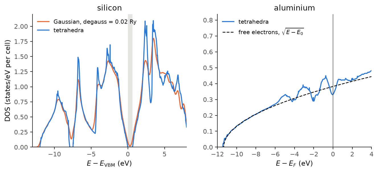
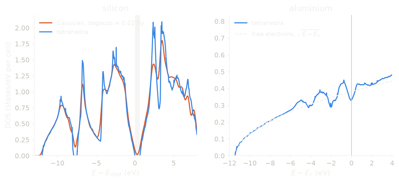
On the left we see silicon on a \(12\times12\times12\) mesh. The grey band is the gap between the highest valence level and the lowest conduction level of this mesh. With tetrahedra, the DOS in the gap is exactly zero. A Gaussian of 0.02 Ry puts states into the gap, 0.02 states/eV at mid-gap, and these states do not exist. The Gaussian also rounds the sharp peaks, which are the van Hove singularities of the bands. So for an insulator, tetrahedra are the better choice.

On the right we see aluminium on a \(16\times16\times16\) mesh, with tetrahedra. Up to about 6 eV below the Fermi level, the DOS follows \(\sqrt{E - E_0}\), the DOS of free electrons in three dimensions (dashed). This is why aluminium is the standard example of a nearly-free-electron metal. Near the Fermi level, the deviations come from the gaps that the lattice potential opens at the zone boundary. The integral of the DOS up to the Fermi level is 3.000001, the three valence electrons of aluminium.

Code of this figure (docs/figures/dos_silicon_aluminium/)

compute.py

"""The DOS of an insulator (silicon) and of a metal (aluminium)."""
import numpy as np
from defuqumat import Calculator
from defuqumat.units import RY_TO_EV
from common import PSEUDO, save

# silicon, with tetrahedra and with a Gaussian of 0.02 Ry
silicon = Calculator.from_file("si.in", pseudo_dir=PSEUDO)
tetra = silicon.get_dos(grid=(12, 12, 12), nbnd=8, scheme="tetrahedra")
gauss = silicon.get_dos(grid=(12, 12, 12), nbnd=8, scheme="gaussian", degauss=0.02)
levels = np.asarray(silicon.dos_states.eigenvalues)
vbm, cbm = levels[:, 3].max(), levels[:, 4].min()

# aluminium, with tetrahedra (the scheme of al.in)
aluminium = Calculator.from_file("al.in", pseudo_dir=PSEUDO)
al = aluminium.get_dos(grid=(16, 16, 16), nbnd=6)
bottom = np.asarray(aluminium.dos_states.eigenvalues).min()

# free electrons, D(E) = c sqrt(E - E0), fitted near the bottom of the band
near = (al.energies > bottom + 0.03) & (al.energies < bottom + 0.30)
slope, intercept = np.polyfit(al.energies[near], al.dos[near] ** 2, 1)
free = np.sqrt(np.maximum(slope * al.energies + intercept, 0.0))

save(si_e=(tetra.energies - vbm) * RY_TO_EV, si_tetra=tetra.dos_ev,
     si_gauss_e=(gauss.energies - vbm) * RY_TO_EV, si_gauss=gauss.dos_ev,
     si_gap=(cbm - vbm) * RY_TO_EV,
     al_e=(al.energies - al.fermi_energy) * RY_TO_EV, al_dos=al.dos_ev,
     al_free=free / RY_TO_EV, al_states_below_ef=al.states_below(al.fermi_energy))

plot.py

"""The DOS of silicon (tetrahedra and Gaussian) and of aluminium."""
import numpy as np
import style

d = np.load("data.npz")


def draw():
    fig, (a, b) = style.figure(2)
    a.axvspan(0.0, d["si_gap"], color=style.ink2(), alpha=0.15, lw=0)
    a.plot(d["si_gauss_e"], d["si_gauss"], color=style.color(1),
           label="Gaussian, degauss = 0.02 Ry")
    a.plot(d["si_e"], d["si_tetra"], color=style.color(0), label="tetrahedra")
    a.set_xlim(-13.0, 8.0)
    a.set_xlabel(r"$E - E_{\rm VBM}$ (eV)")
    a.set_ylabel("DOS (states/eV per cell)")
    a.set_title("silicon")

    b.plot(d["al_e"], d["al_dos"], label="tetrahedra")
    b.plot(d["al_e"], d["al_free"], **style.reference(),
           label=r"free electrons, $\sqrt{E-E_0}$")
    style.zero_line(b, vertical=True)
    b.set_xlim(-12.0, 4.0)
    b.set_xlabel(r"$E - E_F$ (eV)")
    b.set_title("aluminium")
    for ax in (a, b):
        ax.set_ylim(bottom=0.0)
        ax.legend(loc="upper left")
    return fig


style.main(draw)

The projected density of states

Let us now ask which atom and which orbital a state belongs to. We answer it by projecting each Kohn-Sham state on the atomic orbitals \(\phi_i\), which are in the pseudopotential file:

\[ D_i(E) = \sum_{n\mathbf k} w_{\mathbf k}\, \left|\langle\tilde\phi_i|\hat S|\psi_{n\mathbf k}\rangle\right|^2\, \delta(E - \varepsilon_{n\mathbf k}), \qquad |\tilde\phi\rangle = O^{-1/2}|\phi\rangle,\quad O_{ij} = \langle\phi_i|\hat S|\phi_j\rangle . \]

We first make the orbitals orthonormal, which is the Löwdin construction, so the weights of one state add up to at most one. \(\hat S\) is the overlap operator of an ultrasoft or PAW dataset, and the identity for a norm-conserving one. This is the same projection as projwfc.x of Quantum ESPRESSO. The integral of \(D_i\) up to the Fermi level is the Löwdin charge of orbital \(i\). The part of the occupied states that the atomic orbitals cannot describe is the spilling parameter:

\[ \text{spilling} = 1 - \frac{1}{N_{\rm elec}}\sum_i\int^{E_F} D_i(E)\,dE . \]

A small spilling means that the atomic orbitals are a good language for the bonds of this crystal. The orbital character of the states is what X-ray absorption and resonant photoemission see. Here we take silicon with an ultrasoft dataset:

silicon = Calculator.from_file("docs/figures/dos_pdos/si-us.in",
                               pseudo_dir="tests/data/pseudo")
pdos = silicon.get_pdos()

print(pdos.charges.format(("Si",)))
s = pdos.select(l="s")              # both atoms, states/Ry
p1 = pdos.select(atom=0, l="p")     # the first atom only

Lowdin Charges:
     Atom #   1 (Si): total charge =   3.9647
       s =   1.1596
       p =   2.8051, pz=  0.9350, px=  0.9350, py=  0.9350
     Atom #   2: total charge =   3.9647
       s =   1.1596
       p =   2.8051, pz=  0.9350, px=  0.9350, py=  0.9350
     Spilling Parameter:   0.0088

get_pdos takes the same grid, nbnd, scheme and degauss as get_dos. pdos.select(atom=..., l=..., species=..., m=...) sums the channels that match, and l can be a number or a letter. pdos.total is the normal DOS on the same energies. pdos.charges holds the Löwdin charges: charges.total per atom, charges.charges per atom and \(l\), and charges.spilling. pdos.plot(by="l") draws the projections by angular momentum, and you can also choose by="shell" or by="species". For a spin-orbit run, the channels are resolved by \(j\) and \(m_j\) instead of \(m\).

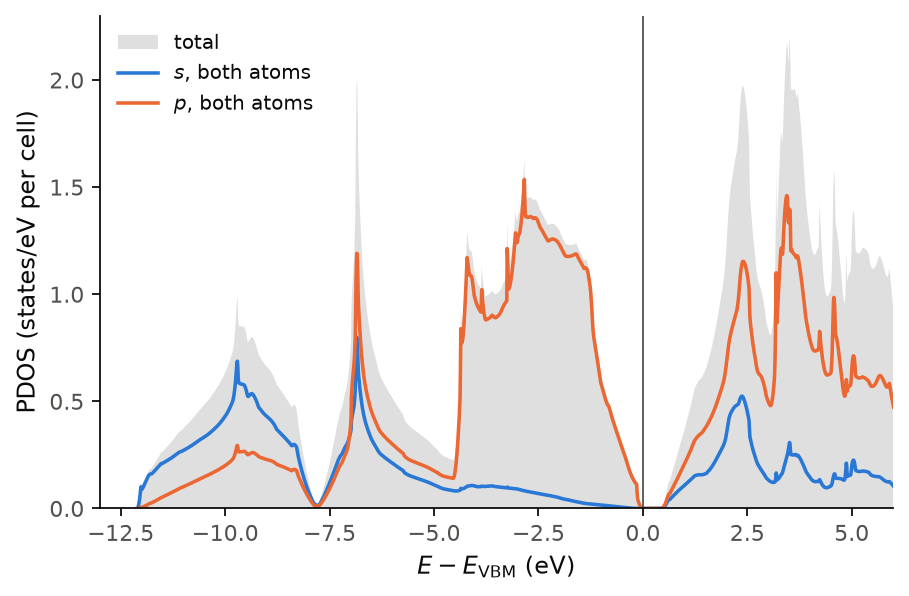
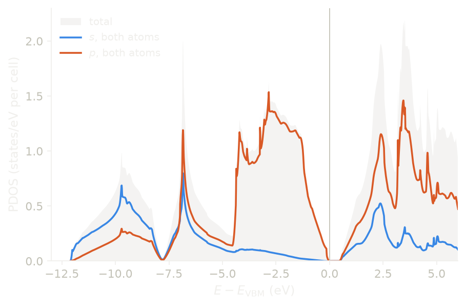
The figure shows silicon with an ultrasoft dataset, on a \(12\times12\times12\) mesh with tetrahedra, and the grey area is the total DOS. We see that the bottom of the valence band, from \(-12\) to about \(-8\) eV, is mostly \(s\), and the top, from about \(-4\) eV to the gap, is almost only \(p\). In between, the two mix. This is the \(sp^3\) picture of a covalent semiconductor, here read from the projections. The conduction band is mostly \(p\) too. The coloured curves sum to slightly less than the total, and the difference is the spilling, 0.9% of the valence charge here.

Code of this figure (docs/figures/dos_pdos/)

compute.py

"""The projected DOS of silicon (ultrasoft), by angular momentum."""
import numpy as np
from defuqumat import Calculator
from defuqumat.units import RY_TO_EV
from common import PSEUDO, save

silicon = Calculator.from_file("si-us.in", pseudo_dir=PSEUDO)
pdos = silicon.get_pdos(grid=(12, 12, 12), nbnd=8, scheme="tetrahedra")

save(energies=(pdos.energies - pdos.fermi_energy) * RY_TO_EV,
     total=pdos.total.dos_ev,
     s=pdos.select(l="s") / RY_TO_EV, p=pdos.select(l="p") / RY_TO_EV,
     charges=np.asarray(pdos.charges.total), spilling=pdos.charges.spilling)

plot.py

"""The projected DOS of silicon: s and p of both atoms over the total."""
import numpy as np
import style

d = np.load("data.npz")


def draw():
    fig, ax = style.figure()
    e = d["energies"]
    ax.fill_between(e, d["total"], color=style.ink2(), alpha=0.18, lw=0, label="total")
    ax.plot(e, d["s"], label=r"$s$, both atoms")
    ax.plot(e, d["p"], label=r"$p$, both atoms")
    style.zero_line(ax, vertical=True)
    ax.set_xlim(-13.0, 6.0)
    ax.set_ylim(bottom=0.0)
    ax.set_xlabel(r"$E - E_{\rm VBM}$ (eV)")
    ax.set_ylabel("PDOS (states/eV per cell)")
    ax.legend(loc="upper left")
    return fig


style.main(draw)

Limits

The projected density of states works with K_POINTS gamma. It agrees with an explicit \(k = 0\) to 4e-12.

The tetrahedron schemes need an automatic k-mesh. If you do not give grid and the SCF used an explicit list of k-points, tetrahedra give an error, because a list of points carries no tetrahedra.

A noncollinear run is symmetrized, with the spin rotated together with the orbitals. A spin-orbit run (lspinorb) is symmetrized too when it is not magnetic. A magnetic spin-orbit run with symmetry gives an error. For it you run with nosym = .true. and the full k-mesh, which is the same physics, or pass symmetrize=False.

A noncollinear run, with or without spin-orbit coupling, has no \(m\)-resolved charges, and charges.charges_lm is None. The charges per atom and per \(l\), charges.charges, are still there.

A fully relativistic dataset with lspinorb = .false. gives an error in the projection, because its channels would be resolved by \(j\) and still be labelled as up and down. So you run it with lspinorb = .true., which is what a fully relativistic dataset is for.

The notebooks for this page are 06, the density of states and 16, the projected density of states.