Electric fields

In this page we put a molecule or a slab in a uniform electric field, we put a crystal in a finite field through the Berry phase, and we compute the polarization of a crystal, with the Born charges that we get from it.

A field across a molecule or a slab

How do we put a uniform field into a periodic cell? A linear potential is not periodic, so we use a saw-tooth, as pw.x does. The potential rises linearly over most of the cell along the reciprocal vector \(\mathbf b_{\rm edir}\), and then it falls back in a thin region of width eopreg, which must be in the vacuum. You switch the field on with tefield = .true., and eamp is its amplitude in Hartree atomic units. edir and emaxpos set its direction and where it falls back.

A molecule or a slab with a dipole creates a field in the vacuum through its periodic images. The dipole correction, dipfield = .true., cancels it by adding a second saw-tooth whose slope follows the dipole of the cell. The energy of the field, for the electrons and the ions together, is:

\[ E_f = \frac{\Omega}{4\pi}\,e^2\Big[-E_{\rm amp}\,D + \tfrac12 D^2\Big], \qquad \frac{\Omega}{4\pi}\,D = \sum_a Z_a\, s(x_a) - \int n(\mathbf r)\, s(x)\, d\mathbf r . \]

Here \(s\) is the saw-tooth, and \(\Omega D/4\pi\) is the dipole of the cell in \(e\,\)bohr. The \(D^2/2\) term is there only with dipfield. The potential and the forces are derivatives of this energy, so a relaxation in a field works. The input is the input of pw.x. Here we take CO in a 10 bohr box with a field of 0.001 Ha a.u. along the bond:

from defuqumat import Calculator

co = Calculator.from_file("docs/figures/electric-field_dipole/co.in",
                          pseudo_dir="tests/data/pseudo")
scf = co.get_scf()
print(f"dipole        {scf.efield_dipole:+.5f} e bohr")
print(f"field energy  {scf.efield_energy:.4e} Ry")
print(co.get_forces().forces[:, 2])     # along the field, Ry/bohr

dipole        -0.03376 e bohr
field energy  8.1848e-05 Ry
[ 0.11696953 -0.11696953]

The code warns that the run uses no symmetry, because a field breaks the symmetry, and pw.x does the same. scf.efield_dipole is the dipole of the cell, and scf.efield_energy is \(E_f\), which is part of the total energy. We see that the two forces are equal and opposite. The field pulls the ions and the electrons in opposite directions, so it stretches or compresses the bond.

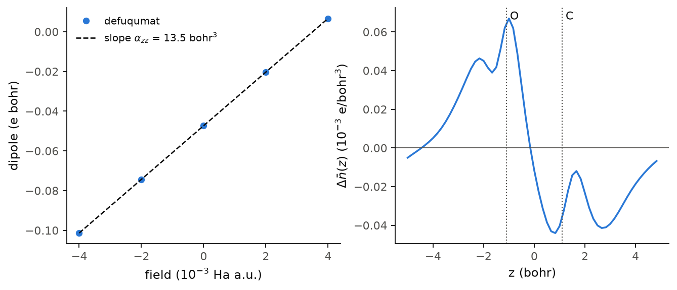
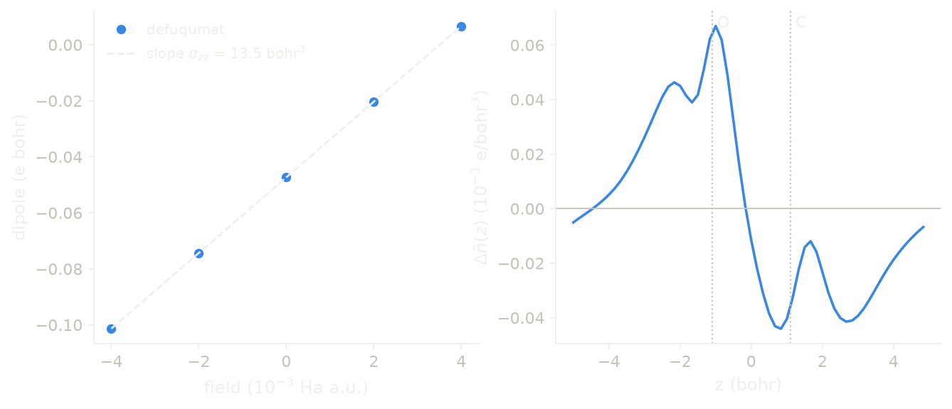
The left panel shows the dipole at five fields. It is linear in the field, and its slope is the polarizability along the bond, \(\alpha_{zz} = 13.5\) bohr\(^3\). The measured static polarizability of CO along the bond is about 15.6 bohr\(^3\). The number here is a rough estimate, because the box is small and the cutoff is low. The right panel shows the change of the electron density, averaged over the \(xy\) plane, when the field goes from 0 to 0.004 Ha a.u. The electrons move towards \(-z\), to the oxygen side, against the field, and the change is zero far from the molecule.

Code of this figure (docs/figures/electric-field_dipole/)

compute.py

"""The dipole of CO against the field, and where the charge goes."""
import numpy as np
from defuqumat import Calculator
from common import PSEUDO, save

text = open("co.in").read()
fields = np.array([-0.004, -0.002, 0.0, 0.002, 0.004])       # Ha a.u.

dipole, force, density = [], [], []
for eamp in fields:
    calc = Calculator.from_text(text.replace("eamp=0.001", f"eamp={eamp}"),
                                pseudo_dir=PSEUDO)
    scf = calc.get_scf()
    dipole.append(scf.efield_dipole)                          # e bohr
    force.append(calc.get_forces().forces[0, 2])              # on O, Ry/bohr
    density.append(np.asarray(scf.density).sum(axis=0).mean(axis=(0, 1)))
    print(f"E = {eamp:+.3f}   p = {dipole[-1]:+.5f} e bohr   F(O) = {force[-1]:+.6f}",
          flush=True)

length = float(calc.system.cell.at[2, 2])
save(fields=fields, dipole=np.array(dipole), force=np.array(force),
     z=np.arange(len(density[0])) * length / len(density[0]), density=np.array(density))

plot.py

"""The dipole of CO against the field, and the change of the density along z."""
import numpy as np
import style

d = np.load("data.npz")
e, p = d["fields"], d["dipole"]
slope, offset = np.polyfit(e, p, 1)
z = d["z"]
z = np.where(z > z[-1] / 2, z - z[-1] - z[1], z)        # the molecule in the middle
order = np.argsort(z)
change = (d["density"][-1] - d["density"][2]) * 1e3      # E = 0.004 minus E = 0


def draw():
    fig, (a, b) = style.figure(2)
    a.plot(e * 1e3, p, "o", label="defuqumat")
    a.plot(e * 1e3, slope * e + offset, **style.reference(),
           label=r"slope $\alpha_{zz}$ = %.1f bohr$^3$" % slope)
    a.set_xlabel(r"field (10$^{-3}$ Ha a.u.)")
    a.set_ylabel(r"dipole (e bohr)")
    a.legend()
    b.plot(z[order], change[order])
    style.zero_line(b)
    for atom, pos in (("O", -1.1), ("C", 1.1)):
        b.axvline(pos, color=style.ink2(), ls=":", lw=1)
        b.text(pos, 0.95, " " + atom, transform=b.get_xaxis_transform())
    b.set_xlabel("z (bohr)")
    b.set_ylabel(r"$\Delta\bar n(z)$ (10$^{-3}$ e/bohr$^3$)")
    return fig


style.main(draw)

A finite field in a crystal

Let us now put a field in a crystal. In a crystal there is no vacuum, so the saw-tooth has nowhere to fall back. We also cannot add \(-e\mathbf E\cdot\mathbf r\) to the Hamiltonian, because \(\mathbf r\) is not periodic. So we minimize the electric enthalpy instead (Souza, Iniguez and Vanderbilt, arXiv:cond-mat/0205633):

\[ F[\psi] = E_{\rm KS}[\psi] - \Omega\,\mathbf E\cdot\mathbf P[\psi] . \]

\(\mathbf P\) is the Berry-phase polarization of the occupied bands, which we compute below. Its derivative with respect to the wavefunctions couples each k-point to its two neighbours on a string of k-points along the field. This is lelfield of pw.x, with the same input: efield in Ry atomic units, gdir the direction, nppstr the points of a string, and an explicit list of k-points. We switch the field on from a converged state without field, which is what pw.x does too.

import numpy as np

folder = "docs/figures/electric-field_dipole/"
ground = Calculator.from_file(folder + "si8-nofield.in",
                              pseudo_dir="tests/data/pseudo").get_scf()
text = open(folder + "si8-field.in").read()

dipole = {}
for e in (-0.001, 0.001):
    run = Calculator.from_text(text.replace("efield=0.001", f"efield={e}"),
                               pseudo_dir="tests/data/pseudo")
    scf = run.get_scf(starting_from=ground)
    dipole[e] = scf.berry_dipoles[0]       # electronic part, Ry a.u.
    print(f"E = {e:+.3f}   p_el = {dipole[e]:.6f}")

volume = float(run.system.cell.volume)
chi = (dipole[0.001] - dipole[-0.001]) / 0.002 / volume
print(f"eps_inf = {1 + 4 * np.pi * chi:.2f}")

E = -0.001   p_el = -0.929969
E = +0.001   p_el = 0.929969
eps_inf = 12.08

scf.berry_dipoles holds the electronic dipole, the ionic dipole and the number of \(2\pi\) jumps of the phase, in Ry atomic units. The slope of the electronic dipole is the susceptibility, and \(\varepsilon_\infty = 1 + 4\pi\chi\). In Ry atomic units the dipole and the field each carry a factor \(\sqrt2\), and the two cancel. The measured \(\varepsilon_\infty\) of silicon is 11.7, and LDA gives a larger value because its gap is too small. This mesh of \(3\times3\times7\) points is also not converged. The page about phonons computes \(\varepsilon_\infty\) from linear response, with no field at all.

The field must stay below the breakdown field of the k-mesh. Above it, electrons can tunnel from the valence to the conduction band between neighbouring k-points, and the enthalpy has no minimum.

The Berry-phase polarization

We now compute the polarization of a crystal. The polarization of a crystal is not the dipole of its unit cell, because that dipole depends on where you cut the cell. What is a property of the crystal is a phase, the Berry phase that the occupied bands collect when \(\mathbf k\) crosses the zone once along \(\mathbf b_i\) (King-Smith and Vanderbilt):

\[ \Omega\,\mathbf P = \sum_i \frac{\varphi_i}{2\pi}\,\mathbf a_i, \qquad \varphi_i = \operatorname{Im}\ln \prod_j \det M(\mathbf k_j, \mathbf k_{j+1}) + 2\pi\sum_a Z_a\, s_{ai} . \]

\(M\) is the matrix of overlaps of the occupied states at two neighbouring k-points. The first term is the electronic phase, and the second the ionic one, with \(s_{ai}\) the crystal coordinate of atom \(a\). The phase is defined modulo \(2\pi\), so \(\mathbf P\) is defined only modulo a quantum. Moving one electron by one lattice vector changes the dipole of the cell by exactly this quantum, and the crystal is the same. What is physical is a difference of \(\mathbf P\) between two structures, on the same branch. This is what a ferroelectric hysteresis loop measures, and it gives the Born charges and the piezoelectric tensor. Here we take AlAs and compute it with alas.get_polarization() on more and more strings:

alas = Calculator.from_file(folder + "alas.in", pseudo_dir="tests/data/pseudo")
for n in (2, 4, 6, 8):
    pol = alas.get_polarization(transverse=(n, n))
    print(f"{n}x{n} strings: electronic {pol.electronic_phase:+.5f}   "
          f"P = {pol.polarization_si:+.5f} C/m^2")
print(f"ionic {pol.ionic_phase:+.5f}, modulo {pol.quantum:.0f}, "
      f"or {pol.quantum_si:.5f} C/m^2")

2x2 strings: electronic +0.00876   P = -0.34909 C/m^2
4x4 strings: electronic -0.00184   P = -0.36444 C/m^2
6x6 strings: electronic -0.00331   P = -0.36657 C/m^2
8x8 strings: electronic -0.00355   P = -0.36691 C/m^2
ionic -0.25000, modulo 1, or 1.44708 C/m^2

get_polarization() reads lberry, gdir and nppstr from the input, as in pw.x, and you can also pass them as keywords. Here gdir counts from 0, so gdir=2 is the third reciprocal vector. transverse=(n1, n2) sets the number of strings in the two other directions, \(4\times4\) if you do not give it. The phases are in units of \(2\pi\), and pol.quantum_si is the quantum in C/m\(^2\).

We see that the ionic phase is exactly \(-1/4\), modulo 1. The electronic phase is small, and it needs enough strings. On \(2\times2\) strings, the mesh of notebook 34, it has the wrong sign. From \(6\times6\) to \(8\times8\) it moves by \(2.4\times10^{-4}\), so \(P\) is converged to about 0.3 mC/m\(^2\). AlAs has no inversion center, so its phase is not fixed by symmetry. In a crystal with inversion, the phase is 0 or half a quantum.

Let us now use a difference of \(\mathbf P\), which is what is physical. If we move one sublattice by \(u\), the polarization changes linearly in \(u\), and the slope is the Born effective charge, the dipole that an atom creates per unit of its displacement:

\[ Z^*_{a,ij} = \frac{\Omega}{e}\,\frac{\partial P_i}{\partial u_{aj}} . \]

In a purely ionic picture \(Z^*\) would be the formal charge of the ion, +3 for Al and \(-3\) for As. It differs from it because the electrons follow the moving atom only in part, so \(Z^*\) says how covalent the bond is. It enters the infrared absorption of the crystal and the LO-TO splitting of its phonons. We take AlAs, move the Al or the As sublattice along \(x\) with alas.with_positions(), and compute get_polarization() at each step. From \(\Omega\,\mathbf P\cdot\mathbf b_3 = \varphi_3\), with the phase in radians, so \(2\pi\) times the printed phase, we get \(\Omega P_x\), since \(\mathbf P\) is along \(x\) for a displacement along \(x\) in this cubic crystal.

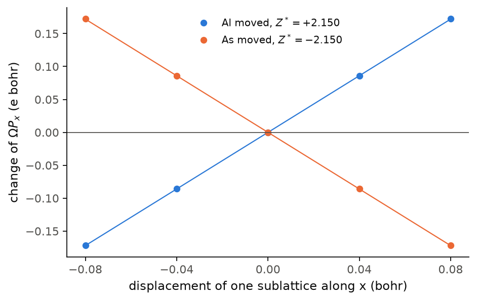
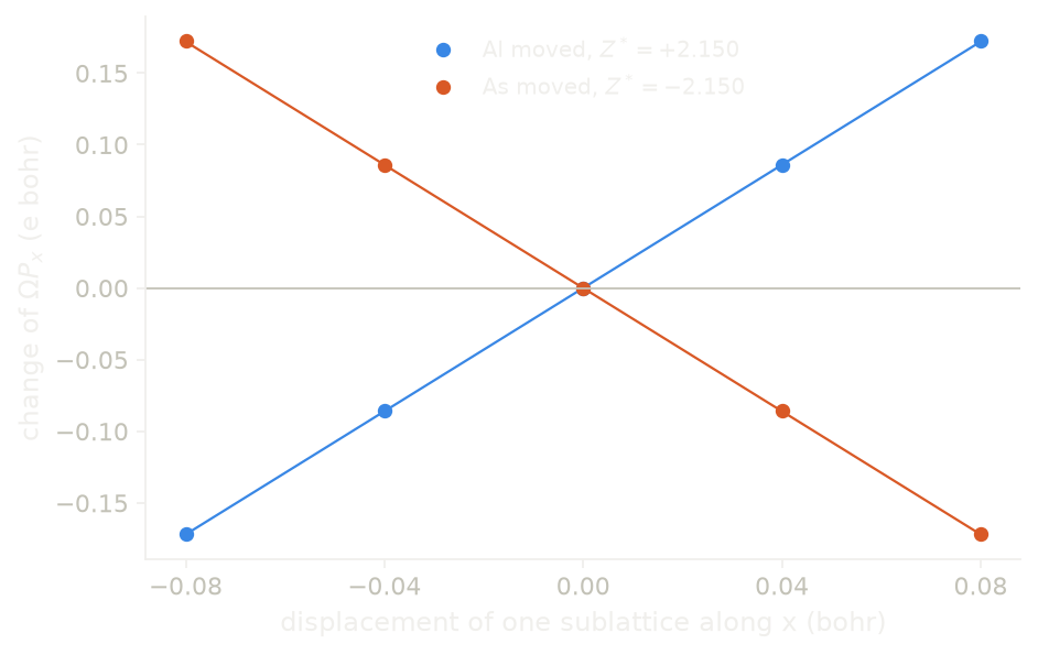
We see two straight lines, and the slopes are the Born charges, \(Z^*_{\rm Al} = +2.150\) and \(Z^*_{\rm As} = -2.150\), on \(8\times8\) strings. On \(4\times4\) strings they are +2.152 and \(-2.152\), so the slope converges much faster than the polarization itself, whose electronic phase moved by \(1.7\times10^{-3}\) between the same two meshes in the table above. Over the five points the largest deviation from the straight line is \(1.3\times10^{-4}\) e bohr, so up to 0.08 bohr the response is linear. The two charges add up to zero, to \(5\times10^{-5}\). This is the acoustic sum rule: moving the As sublattice by \(u\) gives the same crystal as moving the Al sublattice by \(-u\), up to a rigid translation, which changes no dipole. So here the sum rule checks that the Berry phase does not change under a rigid translation of the crystal. The two values are much smaller in size than the formal charge 3, so the bond of AlAs is far from ionic.

Code of this figure (docs/figures/electric-field_born/)

compute.py

"""The polarization of AlAs against the displacement of each sublattice."""
import numpy as np
from defuqumat import Calculator
from common import PSEUDO, save

alas = Calculator.from_file("alas.in", pseudo_dir=PSEUDO)
positions = np.asarray(alas.system.structure.positions)    # bohr
b = np.asarray(alas.system.cell.bg)                         # reciprocal vectors, 1/bohr
u = np.linspace(-0.08, 0.08, 5)                             # bohr, along x
strings = (4, 8)

# the dipole of the cell along x, Omega P_x, from Omega P . b = 2 pi phase
dipole = np.zeros((2, len(strings), len(u)))               # (atom, strings, u)
for atom in (0, 1):
    for i, du in enumerate(u):
        moved = positions.copy()
        moved[atom, 0] += du
        shifted = alas.with_positions(moved)
        for j, n in enumerate(strings):
            pol = shifted.get_polarization(transverse=(n, n))
            dipole[atom, j, i] = 2 * np.pi * pol.total_phase / b[pol.gdir, 0]
        print(f"atom {atom}  u = {du:+.2f} bohr  dipole {dipole[atom, :, i]} e bohr",
              flush=True)

slopes = np.array([[np.polyfit(u, dipole[a, j], 1)[0] for j in range(len(strings))]
                   for a in (0, 1)])
print("Born charges (Al, As) on 4x4 and 8x8 strings:", slopes)
save(u=u, dipole=dipole, slopes=slopes, strings=np.array(strings))

plot.py

"""The change of the dipole of AlAs when one sublattice moves, and the Born charges."""
import numpy as np
import style

d = np.load("data.npz")
u, dipole, slopes = d["u"], d["dipole"], d["slopes"]


def draw():
    fig, ax = style.figure()
    for atom, name in ((0, "Al"), (1, "As")):
        change = dipole[atom, -1] - dipole[atom, -1][len(u) // 2]     # 8x8 strings
        ax.plot(u, change, "o", color=style.color(atom),
                label=f"{name} moved, $Z^* = {slopes[atom, -1]:+.3f}$")
        ax.plot(u, slopes[atom, -1] * u, color=style.color(atom), lw=1.0)
    style.zero_line(ax)
    ax.set_xlabel("displacement of one sublattice along x (bohr)")
    ax.set_ylabel(r"change of $\Omega P_x$ (e bohr)")
    ax.set_xticks([-0.08, -0.04, 0.0, 0.04, 0.08])
    ax.legend(loc="upper center")
    return fig


style.main(draw)

Limits

With a saw-tooth field (tefield), the stress gives an error, so a vc-relax is not possible, and pw.x also switches the stress off with this field. Linear response, real-time propagation and the ultracell give an error too, because they have not been checked with the field. A charged plate (gate) gives an error, because it needs a charged cell and a nonzero tot_charge gives an error. dipfield without tefield gives an error, because in pw.x it does nothing. As in pw.x, the run uses no symmetry, and the code warns about it.

A finite field by the Berry phase (lelfield) gives an error for an ultrasoft or PAW dataset, because the overlap between two k-points then needs the augmentation, and the force needs its derivative. It works for nspin = 2 when the two channels hold the same number of electrons (tot_magnetization = 0). It gives an error for a collinear magnet, because pw.x counts the occupied bands of a channel as nelec/2, so there is no number to check against. It works for a spinor run without spin-orbit coupling, with or without a magnetization, and for a spin spiral. For a spiral, each spinor component is moved along the string on its own sphere. We checked a spiral against its commensurate supercell, and the supercell against pw.x. Spin-orbit coupling gives an error. A streamed wavefunction store (wfc_store = 'stream') works, and k-point pools give an error. Only occupations = 'fixed' is accepted, so smearing or from_input gives an error, even for an insulator, because a Berry phase belongs to a gapped set of bands. With an automatic k-mesh, pw.x reads the field from efield_cart and ignores efield and gdir. This works when efield_cart points along one Cartesian axis and the other two lattice vectors have no component along it. efield_cart in more than one direction gives an error, and so does an automatic mesh with efield_cart zero, which in pw.x is a run with no field. A cell where \(\mathbf a_g\) is not along the Cartesian axis \(g\) gives an error. The stress gives an error, and the field terms of the stress are not in pw.x either. DFT+U, tefield at the same time, gamma-only storage, every linear response, real-time propagation and the ultracell give an error too.

The Berry-phase polarization gives an error for a metal, because a smeared occupation does not say which bands the string carries. For nspin = 2 each spin channel has its own strings, and the two phases add, as in pw.x. The quantum is then 1. This needs occupations = 'fixed' with tot_magnetization, and from_input gives an error. A spin spiral gives an error, because its two spinor components live on spheres centred at \(\mathbf k \pm \mathbf q/2\). It works for a spinor run (noncolin), where the quantum is half the scalar one because a spinor band holds one electron, and for ultrasoft and PAW datasets.

The notebooks for this page are 53, a molecule in an electric field, 54, silicon in a finite electric field and 34, electric polarization.