DFT+U

In this page we add a Hubbard \(U\) to a localized shell, here the \(3d\) shell of iron in FeO, and we see what it does to the occupations and to the density of states.

The Hubbard correction

We start with what goes wrong without \(U\). LDA and GGA spread the electrons of a localized \(d\) or \(f\) shell too evenly over its orbitals, so they often make a metal of an oxide that is an insulator. DFT+U adds an energy that is zero when each orbital of the shell is full or empty, and positive in between. In the simplest form (Dudarev) it is:

\[ E_U = \sum_{I,\sigma} \frac{U^I}{2}\, \mathrm{Tr}\Big[ n^{I\sigma} \big( 1 - n^{I\sigma} \big) \Big], \qquad n^{I\sigma}_{mm'} = \sum_{n\mathbf k} f_{n\mathbf k\sigma} \langle \psi_{n\mathbf k\sigma} | \hat S | \varphi^I_{m'}\rangle \langle \varphi^I_{m} | \hat S | \psi_{n\mathbf k\sigma}\rangle . \]

Here \(n^{I\sigma}\) is the occupation matrix of the shell on atom \(I\), the projection of the occupied states on its atomic orbitals \(\varphi^I_m\). The potential of \(E_U\) pushes the occupied orbitals down and the empty ones up, by about \(U/2\) each. This is the physics of a Mott insulator that the functional misses, and photoemission and inverse photoemission see the gap between the two.

You give \(U\) in the HUBBARD card of pw.x, in eV:

HUBBARD {atomic}
U Fe1-3d 4.3
U Fe2-3d 4.3

The projectors are atomic, ortho-atomic or norm-atomic. A value of \(U\) is only meaningful together with the projectors it was chosen for. Here we take antiferromagnetic FeO, with the moments of the two iron atoms opposite, and we compute its ground state with get_scf():

from defuqumat import Calculator

folder = "docs/figures/dft-plus-u_feo/"
feo = Calculator.from_file(folder + "feo.in", pseudo_dir="tests/data/pseudo")
scf = feo.get_scf()
print(f"total energy {scf.total_energy:.8f} Ry")
print(f"Hubbard term {scf.energy_terms['hubbard']:.8f} Ry")
for atom, (up, down, total) in scf.hubbard_occupations.items():
    print(f"atom {atom + 1}: Tr n = {up:.4f} up, {down:.4f} down")

total energy -174.47156068 Ry
Hubbard term 0.31370438 Ry
atom 3: Tr n = 4.9911 up, 1.8454 down
atom 4: Tr n = 1.8454 up, 4.9911 down

scf.energy_terms["hubbard"] is \(E_U\), and it is part of the total energy. scf.hubbard_occupations gives, for each atom with a \(U\), the traces of \(n^{I\uparrow}\) and \(n^{I\downarrow}\) and their sum. scf.ns is the occupation matrix itself, with the axes (spin, atom, \(m\), \(m'\)). We see that atom 3 has 4.99 electrons in its majority shell and 1.85 in its minority shell, and atom 4 is its mirror image. The forces and the stress include the Hubbard term.

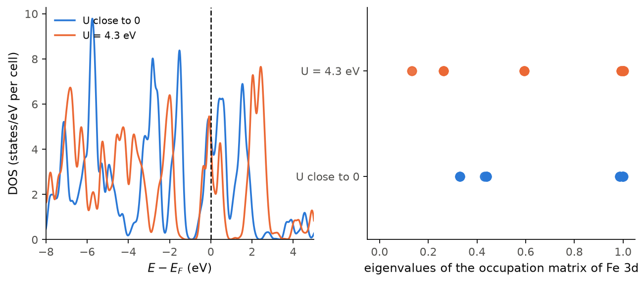
In the right panel we see what \(U\) does. The eigenvalues of the occupation matrix are the occupations of the natural orbitals of the shell. With \(U = 4.3\) eV they move towards 0 and 1, and their mean distance from the nearer of 0 and 1 falls from 0.200 to 0.148. The left panel shows the DOS of the cell. \(U\) pushes the empty minority \(d\) states up, to about 2 eV, and the occupied \(d\) states down. But a narrow peak stays at the Fermi level, so this run is still a metal. The reason is the one minority \(d\) electron of Fe\(^{2+}\). In this cell it is shared by a pair of degenerate orbitals, with 0.59 in each. As long as the symmetry keeps the two orbitals equal, \(U\) cannot fill one and empty the other. To get the insulator, we must break this degeneracy, for example with a lower symmetry or a starting occupation (starting_ns_eigenvalue, as in pw.x). The run above uses neither.

Code of this figure (docs/figures/dft-plus-u_feo/)

compute.py

"""FeO with U = 4.3 eV and with U close to zero: the DOS and the occupations."""
import numpy as np
from defuqumat import Calculator
from defuqumat.units import RY_TO_EV
from common import PSEUDO, save

text = open("feo.in").read()
out = {}
for name, t in (("U", text), ("noU", text.replace("-3d 4.3", "-3d 1.d-8"))):
    calc = Calculator.from_text(t, pseudo_dir=PSEUDO)
    scf = calc.get_scf(max_iterations=200)
    dos = calc.get_dos(grid=(6, 6, 6), nbnd=24)
    ns = np.asarray(scf.ns)                       # (spin, Fe site, 5, 5)
    out[name + "_e"] = (dos.energies - dos.fermi_energy) * RY_TO_EV
    out[name + "_dos"] = dos.total_dos / RY_TO_EV
    out[name + "_occ"] = np.linalg.eigvalsh(ns).ravel()     # natural occupations
    out[name + "_energy"] = scf.total_energy
    print(name, f"E = {scf.total_energy:.9f} Ry in {scf.iterations} iterations", flush=True)

save(**out)

plot.py

"""FeO: the total DOS, and the eigenvalues of the occupation matrices."""
import numpy as np
import style

d = np.load("data.npz")


def draw():
    fig, (a, b) = style.figure(2)
    for k, (name, label) in enumerate((("noU", "U close to 0"), ("U", "U = 4.3 eV"))):
        a.plot(d[name + "_e"], d[name + "_dos"], color=style.color(k), label=label)
        b.plot(d[name + "_occ"], np.full(d[name + "_occ"].size, k), "o",
               color=style.color(k), alpha=0.7, ms=8)
    a.axvline(0.0, **style.reference())
    a.set_xlim(-8.0, 5.0)
    a.set_ylim(bottom=0.0)
    a.set_xlabel(r"$E - E_F$ (eV)")
    a.set_ylabel("DOS (states/eV per cell)")
    a.legend(loc="upper left")
    b.set_yticks([0, 1], ["U close to 0", "U = 4.3 eV"])
    b.set_ylim(-0.6, 1.6)
    b.set_xlim(-0.05, 1.05)
    b.set_xlabel("eigenvalues of the occupation matrix of Fe 3d")
    return fig


style.main(draw)

The full interaction, and the double counting

Let us now go beyond a single \(U\). \(U\) alone is the cost of two electrons in the same shell, and it does not say which two. Hund's rule says that two electrons in different orbitals with parallel spins cost less. To describe this, you add a J on the card, which asks for the full interaction of the shell, built from the Slater integrals \(F^0 = U\), \(F^2\) and \(F^4\):

HUBBARD {atomic}
U Fe1-3d 4.3
J Fe1-3d 1.0

The functional already counts part of the interaction, and the double counting removes it. You choose how with hubbard_double_counting. The fully localized limit ('fll', the default) assumes that each orbital is full or empty, which fits a magnetic insulator. Around mean field ('amf') assumes that the shell is filled evenly, so an even shell gets no correction:

for name in ("feo-fll.in", "feo-amf.in"):
    scf = Calculator.from_file(folder + name, pseudo_dir="tests/data/pseudo").get_scf()
    print(f"{name}: E_U = {scf.energy_terms['hubbard']:+.4f} Ry")

feo-fll.in: E_U = +0.2321 Ry
feo-amf.in: E_U = -0.0052 Ry

The two runs have the same \(U\) and \(J\), and only the double counting differs. We see that \(E_U\) changes from 0.23 Ry to almost nothing. Which one to use is a statement about the material.

With hubbard_slater = 'yukawa' the code computes \(F^2\), \(F^4\) and \(J\) from the radial function of the shell itself, with a screened Coulomb interaction. The screening length is chosen so that \(F^0\) is the \(U\) on the card. This needs a PAW dataset, because only PAW has the all-electron partial wave.

Fixing a tensor moment

The occupation matrix of a shell can also be written as a sum of multipoles, the tensor moments \(w^{kpr}_t\), with \(k\) the rank in the orbital index, \(p\) the rank in spin and \(r\) their coupling. The charge is \(w^{000}\), the spin moment is \(w^{011}\), and \(\mathbf{L}\cdot\mathbf{S}\) is \(w^{110}_0\). With a TENSOR_MOMENTS card you fix one of them, and the SCF converges to a state that carries it, which selects an orbital or multipolar order that the SCF would not find on its own:

&system
   tensor_moment_penalty = 20.0
/
TENSOR_MOMENTS
 N-2p 1 1 0 0 -0.40      # hold L.S at -0.40

The constraint is a quadratic penalty with strength tensor_moment_penalty, so the moment approaches its target as the penalty grows rather than reaching it. The energy of the penalty is not part of the reported total energy.

Limits

The intersite \(V\) gives an error, and so do background channels (a second manifold on the same species, or hubbard_occ for a second channel), orbital indices on a HUBBARD line (the orbital-resolved form) and the wf and pseudo projectors.

hubbard_double_counting = 'amf' needs the full form of DFT+U, which a J on the card or hubbard_slater = 'yukawa' selects. Without them it gives an error, because the simple form of DFT+U is the fully localized limit itself. ALPHA, J0 or BETA together with a J give an error, as in pw.x. There is no input for Slater or Racah integrals given directly (Elk's inpdftu = 2 and 3), since they are the same three numbers as \(U\), \(J\) and \(B\), and there is no interpolation between the fully localized limit and around mean field.

A collinear DFT+U run needs nosym when its magnetic group has operations combined with time reversal, because these exchange the two spin channels. A spinor run (noncolin = .true.) does not need it.

A fixed tensor moment needs a spinor run, because in a collinear run it reduces to the fixed spin moment that constrained_magnetization already gives.

hubbard_slater = 'yukawa' needs a PAW dataset. A norm-conserving or ultrasoft orbital would give a far too small \(F^0\), so it gives an error. It also gives an error when the partial wave has a norm below 0.7 inside the cutoff, which is by default the augmentation radius of the dataset, and you can set a larger one with hubbard_radial_cutoff. The run keeps, with each manifold, the cutoff it used and the norm inside it, and this norm tells you whether the shell is bound inside the cutoff. J0, ALPHA and BETA give an error with 'yukawa'.

A Hubbard \(U\) gives an error in the force theorem for the anisotropy and in the linear response. The magnons work with the simplified functional. The relaxed anisotropy works.

The notebook for this page is 13, DFT+U.