Total energy and the density

In this page we compute the ground state of a crystal, meaning its total energy and its electron density. Everything else in this guide starts from this ground state.

The Kohn-Sham total energy

We start with the quantity we minimize. The ground state is the minimum of the Kohn-Sham total energy, as a functional of the density \(n(\mathbf r)\):

\[ E[n] = T_s[n] + \int v_{\rm ext}(\mathbf r)\, n(\mathbf r)\, d\mathbf r + E_{\rm H}[n] + E_{\rm xc}[n] + E_{\rm Ewald}. \]

Here \(T_s\) is the kinetic energy of non-interacting electrons with density \(n\), and \(v_{\rm ext}\) is the potential of the ions, in our case a pseudopotential. \(E_{\rm H}\) is the classical Coulomb energy of the density, \(E_{\rm xc}\) is the exchange-correlation energy, which is LDA or a GGA, and \(E_{\rm Ewald}\) is the Coulomb energy of the ions.

The density comes from the occupied Kohn-Sham states:

\[ \left[-\nabla^2 + v_{\rm eff}[n](\mathbf r)\right]\psi_{n\mathbf k} = \varepsilon_{n\mathbf k}\,\psi_{n\mathbf k}, \qquad n(\mathbf r) = \sum_{n\mathbf k} w_{\mathbf k}\, f_{n\mathbf k}\, |\psi_{n\mathbf k}(\mathbf r)|^2 . \]

The equation is in Rydberg units, so the kinetic operator is \(-\nabla^2\). The potential \(v_{\rm eff}\) depends on the density, and the density depends on the states, so the problem is a fixed point, meaning that the density that goes in must be the density that comes out. This is the self-consistent field, or SCF. We start from a sum of atomic densities, solve for the states, build a new density, mix it with the old one, and repeat until the two agree.

Running the SCF

Let us now run the SCF for silicon. We compute it with calc.get_scf():

from defuqumat import Calculator

calc = Calculator.from_file("docs/figures/bands_silicon/si.in",
                            pseudo_dir="tests/data/pseudo")
scf = calc.get_scf()

print(f"converged in {scf.iterations} iterations")
print(f"total energy {scf.total_energy:.8f} Ry")
for name, value in scf.energy_terms.items():
    print(f"{name:<13} {value:>15.8f} Ry")

converged in 7 iterations
total energy -15.83929992 Ry
one-electron       4.79887528 Ry
hartree            1.07474038 Ry
xc                -4.81315700 Ry
ewald            -16.89975858 Ry

The energy terms are the ones pw.x prints, and the four terms add up to the total energy. The one-electron term is the band energy minus the double counting.

The SCF stops when the estimated error of the energy is below conv_thr, in Ry. This has the same meaning as in pw.x, so the two codes stop at the same point. You can set it in the &electrons namelist or as a keyword, calc.get_scf(conv_thr=1e-10). Other keywords of get_scf are mixing_beta, mixing_mode and max_iterations.

The result is stored in calc, so a second call to get_scf() with the same keywords returns it without running again. A call with other keywords runs the SCF again and replaces it.

The density

We now look at the density. It is on the real-space grid of the run, in electrons per bohr\(^3\), and the first axis is the spin channel, which is there also for a spin-unpolarized run:

n = scf.density                        # electrons/bohr^3 on the real-space grid
omega = calc.system.cell.volume        # bohr^3
print(n.shape)
print(f"{float(n.mean()) * float(omega):.6f} electrons in the cell")

(1, 20, 20, 20)
8.000000 electrons in the cell

We see that the integral of the density is the number of valence electrons, four per silicon atom. X-ray diffraction measures the Fourier components of the total density, and we compute these in the page about structure factors.

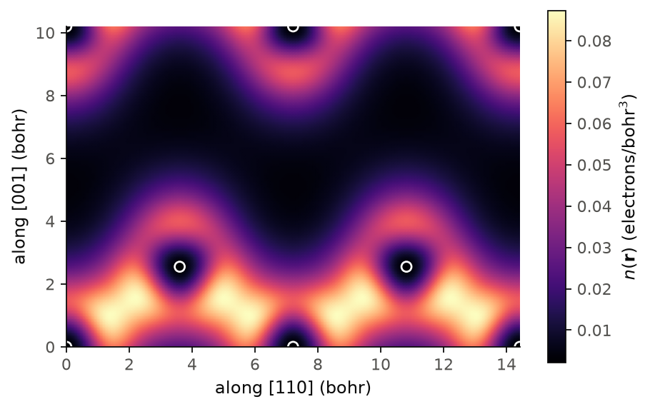
The figure shows the valence density of silicon in the \((1\bar10)\) plane, the plane that holds the zigzag chains of bonds, and the circles are the atoms. We see that the density has its maxima in the middle of the bonds, between two atoms, and not on the atoms, which is the covalent bond of silicon. On the atoms the valence density is small, because the pseudopotential is repulsive inside the core region, so it pushes the valence states out into the bonds. The large dark regions are the open channels of the diamond structure.

Code of this figure (docs/figures/ground-state_density/)

compute.py

"""The valence density of silicon in the (1-10) plane, which holds the bonds."""
import numpy as np
from defuqumat import Calculator
from common import PSEUDO, save

calc = Calculator.from_file("si.in", pseudo_dir=PSEUDO)
scf = calc.get_scf()
rho = np.asarray(scf.density)[0]             # electrons/bohr^3 on the FFT grid
at = np.asarray(calc.system.cell.at)         # lattice vectors in bohr, as rows
alat = calc.system.cell.alat

# the Fourier coefficients: rho(r) = sum_G c_G exp(i G.r)
c = np.fft.fftn(rho).ravel() / rho.size
m = np.meshgrid(*[np.fft.fftfreq(n) * n for n in rho.shape], indexing="ij")
g = np.stack([x.ravel() for x in m], axis=1) @ (2 * np.pi * np.linalg.inv(at).T)

# the plane: [110] across, [001] up, one conventional cell
e1 = np.array([1.0, 1.0, 0.0]) / np.sqrt(2.0)
e2 = np.array([0.0, 0.0, 1.0])
u = np.linspace(0.0, np.sqrt(2.0) * alat, 161)
v = np.linspace(0.0, alat, 115)
image = np.array([((np.exp(1j * (a * e1 + v[:, None] * e2) @ g.T)) @ c).real
                  for a in u])

# the atoms on this plane, from the atoms of nearby cells
cells = np.array([[i, j, k] for i in range(-3, 4) for j in range(-3, 4)
                  for k in range(-3, 4)]) @ at
r = (cells[:, None, :] + np.asarray(calc.system.structure.positions)).reshape(-1, 3)
on = ((abs(r @ [1.0, -1.0, 0.0]) < 1e-6) & (r @ e1 > -1e-6) & (r @ e1 < u[-1] + 1e-6)
      & (r @ e2 > -1e-6) & (r @ e2 < v[-1] + 1e-6))
save(u=u, v=v, density=image, atoms=np.stack([r[on] @ e1, r[on] @ e2], axis=1),
     total_energy=scf.total_energy)

plot.py

"""The valence density of silicon in the (1-10) plane, with the atoms as circles."""
import numpy as np
import style

d = np.load("data.npz")


def draw():
    fig, ax = style.figure()
    mesh = ax.pcolormesh(d["u"], d["v"], d["density"].T, shading="gouraud")
    ax.scatter(d["atoms"][:, 0], d["atoms"][:, 1], s=40, facecolors="none",
               edgecolors="white", lw=1.2)
    ax.set_aspect("equal")
    ax.set_xlabel("along [110] (bohr)")
    ax.set_ylabel("along [001] (bohr)")
    style.colorbar(fig, mesh, ax, r"$n(\mathbf{r})$ (electrons/bohr$^3$)")
    return fig


style.main(draw)

When the SCF does not converge

Most crystals converge with the default mixing, but some cells are hard, for example a metal slab with vacuum, a magnet with a soft direction or a cell with DFT+U. For these we use mixing_mode='robust', which chooses the mixing from the cell and checks every step:

scf = calc.get_scf(mixing_mode="robust")

If the cell has vacuum and a smeared occupation, the mode screens the charge with the local density of states at the Fermi level, and otherwise it uses plain Anderson mixing. Each step is judged by the Kohn-Sham energy of the states that the step produces, which cannot go below the ground-state energy. A step is kept if this energy or the residual goes down, and otherwise the step is cut in half. This is the adaptive damping of Herbst and Levitt (arXiv:2109.14018).

We can also choose the mixing ourselves. mixing_mode='ldos' is the preconditioner of Herbst and Levitt (arXiv:2009.01665) for a metal beside vacuum. It screens the residual with the local density of states at the Fermi level, so it acts as Kerker mixing in the metal, does nothing in the vacuum and is plain Anderson mixing in an insulator, with no parameter to choose. A bulk cell has no charge sloshing to cure, so there we keep anderson.

mixing_mode='adaptive' is the mixer of Elk. It keeps a separate step length for each component of the density, which grows while the residual of that component keeps its sign and is cut when the sign changes. This helps when the SCF crawls rather than overshoots, which is the case of a magnet with a soft direction. Note that in this mode mixing_beta is not a step length but the increment and the floor of the steps. It is 0.05 when mixing_beta is set neither in the input file nor in the call, so the same number means two different things in the two modes, and the 0.7 of a pw.x input is too large here.

mixing_beta_mag gives the magnetization a step length of its own, separate from the mixing_beta of the charge. When it is unset, the magnetization takes mixing_beta, as in pw.x. Whether it helps depends on which channel the run is slow in, and calc.get_scf(residual_split=True) writes into scf.history how much of the residual of each iteration is in the charge and how much is in the magnetization.

scf_solver='newton-krylov' does not mix at all. It solves the condition that the output density equals the input density by Newton's method, and the way the Jacobian is applied is chosen with scf_solver_options={"jvp": ...}. The default "finite-difference" is a central difference of one SCF step and is the fastest. "autodiff" differentiates the eigensolver step by step, and "sternheimer" solves the Sternheimer equation for the response of the converged states, as density-functional perturbation theory does, which is the exact Jacobian. On the cells we measured Newton is slower than mixing, and what it buys is that it converges to the solution it starts nearest, also an unstable one that a mixer cannot hold.

If the SCF reaches max_iterations without converging, the code warns and scf.converged is False. The other methods of calc that start from the ground state then give an error, because they need a converged density.

Limits

K_POINTS gamma asks for the half-sphere storage of the gamma trick, which halves the memory of the wavefunctions. We use it only for a norm-conserving run with nosym = .true., no spinor or spiral and no Hubbard \(U\). Otherwise we run an explicit \(k = 0\) on the full sphere instead, with the same result at twice the cost, and the code warns. For a crystal with symmetry, nosym = .true. is the way to keep the half sphere. calc.estimate() makes the same choice as the run, so it sizes the run either way.

After a run on the half sphere, the following give an error, because their plane-wave sums are not written for it. These are the forces and the stress with method='analytic'. The optical conductivity, the Kerr angle, second-harmonic generation and the shift current still give an error. So does a response to an electric field, which is the dielectric tensor, the Born charges, the Raman tensor and the strain response, and so does the ultracell. For all of these the way out is the same cell at K_POINTS automatic with 1 1 1 0 0 0, which is exact. A Berry-phase field, lelfield, gives an error with K_POINTS gamma, as in pw.x. The dynamical matrix, also a partial one, the topological invariants and a potential-only meta-GGA work on the half sphere.

The projected density of states, the site angular momenta, the absorption spectrum, the transverse spin susceptibility, the STM image, the tunnelling spectrum and both transmissions work on the half sphere. They agree with an explicit \(k = 0\) to 1e-7 or better. The band velocities work on the half sphere too, because the code copies the states onto the whole sphere before it takes \(\partial H/\partial\mathbf k\). So does real-time propagation, where the states are solved again on the whole sphere.

A checkpoint holds the state and not the report of the run. The stress, the solver, the history and the site charges and moments are not stored. A DFT+U state is saved, and its Hubbard manifold is built again from the HUBBARD card when it is loaded. A fixed-spin-moment state is saved with the field that the scheme reached.

A functional that the pseudopotentials name and that we do not implement gives an error, and it is never replaced by LDA.

A converged run does not prove that we found the ground state. On a cell with a soft or degenerate magnetic direction, another mixer or only another mixing_beta can converge to another self-consistent solution, and each reports converged = True. On such a cell we vary both, and compare the energy and scf.site_moments, or cell_moments() of an ultracell result, not only the number of iterations.

The robust mode is not guaranteed to converge. Convergence is proved only for its last step, damped mixing of the Hamiltonian, and the rest is measured. It can also find another solution than plain Anderson. With Marzari-Vanderbilt or Methfessel-Paxton smearing its energy is not a lower bound, so it keeps a step on the residual only, has no last step, and warns. It gives an error for tetrahedra, a potential-only meta-GGA, lelfield, a magnetic field that is updated or reduced during the run, rotate_moments, scf_solver and mixing_beta_mag, which the mode sets itself. It runs with k-point pools and with a checkpoint. A run that continues from a checkpoint takes the same steps as a run that was not stopped. With mixing_from alone, the mixer history is kept and the step control starts again. The ultracell does not take it.

mixing_mode='ldos' screens only the charge, so the magnetization takes mixing_beta and the soft direction of a magnet is not helped. With fixed or from_input occupations there are no states at the Fermi level, so the run is plain Anderson mixing and the code warns. It does not help a metal on a semiconductor or a \(d\)-electron magnet, and on a bulk \(d\)-metal it takes more iterations than anderson. Near a magnetic transition it can also change the state found. On benchmarks/fe-unstable.in it lands on a moment of 0.42 \(\mu_B\), where plain anderson stops at the nonmagnetic state. It also works with tetrahedra. Then the delta at the Fermi level is the derivative of the tetrahedron weights, so no width is needed. On a bulk metal it gives the same energy as anderson, and on the ten-site aluminium cell al10-metal-tetra.in it needs 19 iterations, where pw.x needs 55. It can also be the warmup_mixing of the Newton solver, but not together with tetrahedra, because we have not checked that case. It gives an error in the ultracell and in a response loop. Under scf_solver='newton-krylov' the solver uses Kerker and mixing_mode does not reach it.

Under mixing_mode='adaptive' the code warns when mixing_beta is above 0.5, because the steps then reach their maximum within two iterations and the run is plain linear mixing. Adaptive mixing with a preconditioner gives an error, because its step lengths act point by point in real space. So in the ultracell, where Kerker is on by default, it needs kerker=False.

mixing_beta_mag gives an error with mixing_mode='adaptive', because that mode already has one step length per component, and when it is not positive. It acts on the density only, and the augmentation charge of an ultrasoft or PAW run, the Hubbard occupations and the kinetic-energy density keep mixing_beta. The residual of the augmentation charge is written into scf.history at every iteration as becsum_accuracy, outside the dr2 that decides convergence, so you can ask with a number whether it needs a step of its own.

Under scf_solver='newton-krylov', a fixed occupation that cuts a degenerate multiplet, as the Hund's-rule filling of an atom does, converges, but the code still warns, because the wavefunctions and the band-resolved quantities depend on which members of the multiplet are filled. A smearing is the cure. With "jvp": "autodiff" the Jacobian is not exact at a degenerate band, for example the threefold band of silicon at \(\Gamma\), and it is worse from a cold start and at a tight eigensolver threshold, a factor of 2.3 off at ethr \(=10^{-13}\). The default finite difference starts the eigensolver from the converged states, so it is the derivative of a slightly different map, 5 to 40 per cent off the exact one, and Newton still converges with it. The "sternheimer" Jacobian does not depend on which states fill a degenerate multiplet. "jvp": "sternheimer" gives an error with a Hubbard \(U\), a meta-GGA, a magnetic noncollinear run, wfc_store='host', a fixed occupation that cuts a degenerate multiplet, tetrahedra, from_input occupations, tot_magnetization with a smearing, a spin spiral, a saw-tooth or Berry-phase electric field, and a magnetic field or a constrained moment.

The Newton solver takes tetrahedra and from_input occupations with the default "finite-difference" Jacobian and with "autodiff". On al-tetrahedra.in it gives the total energy of pw.x to 3e-9 Ry. With k-point pools these two occupations give an error, because we have not checked them there. The Newton solver also runs with a uniform magnetic field (B_field) in a collinear run, and with a constrained moment of the kind atomic, atomic direction or total in a noncollinear run. The Newton solver also runs with the field schemes fsm in a collinear run, and atomic fsm and atomic fsm direction in a noncollinear run. Here the field is solved together with the density. The solver stops when the field times the moment error is below conv_thr. This is the error of the total energy, which does not contain the field energy. We measured it with scf_solver_options={"forcing": 0.5, "warmup": 6, "max_iterations": 80} at conv_thr = 1e-11. On fe-fsm.in it stops after 39 steps, and the total energy agrees with the mixing loop to 8e-13 Ry. On a canted iron pair with 8 k-points it needs 63 steps (atomic fsm) and 60 steps (atomic fsm direction). The total energy then agrees with the mixing loop to 7e-13 Ry, or to the mixing loop's own error of 1e-9 Ry for atomic fsm direction. This takes 3 to 5 times the time of the mixing loop. We did not measure the default options of the Newton solver here. With 40 steps or with the defaults the solver can stop before it converges. The mixing loop then takes over and accepts the moment to 1e-3 Bohr magnetons, so the run reports converged while the total energy can be off by 1e-11 to 3e-9 Ry. The code warns when this happens. With fsm_update = 'secant', with fsm in a noncollinear run, with k-point pools, and together with a Hubbard \(U\), a meta-GGA, tetrahedra or from_input occupations, or K_POINTS gamma, it gives an error. It also gives an error for reducebf below 1, because there the field goes to zero, so the solver would solve the problem without the field. It also gives an error for total direction, atomic texture, a LOCAL_MAGNETIC_FIELDS card, a uniform field in a noncollinear run, a constrained moment in a collinear run, and "jvp": "autodiff" with any field, because these are not checked yet. The Newton solver gives an error for a Hubbard \(U\) in a noncollinear run, with or without a field. There the occupation matrix is complex, and the solver keeps only its real part.

The notebooks for this page are 02, silicon and 17, reaching self-consistency.