Magnetic anisotropy

In this page we compute which way a magnet wants to point. We compute the energy against the direction of the moment and the torque, and then we do a self-consistent run that turns its own moment onto the easy axis.

The force theorem

Without spin-orbit coupling the energy of a magnet does not depend on the direction of its moment. Spin-orbit coupling ties the spin to the lattice, and then the energy depends on the direction. The difference between the hard and the easy direction is the magnetocrystalline anisotropy energy. It decides whether a material is a hard magnet, and it is measured by ferromagnetic resonance and torque magnetometry. It is small, about 1 meV in the cobalt below, on a total energy of about 1000 eV, so two separate SCF runs would have to agree in their ninth digit.

The force theorem avoids this. We converge the magnet once without spin-orbit coupling. Then we turn its magnetization to each direction \(\hat{\mathbf n}\) and diagonalize once with the coupling, at this fixed density. The anisotropy is the difference of the band energies:

\[ E(\hat{\mathbf n}) = \sum_{n\mathbf k} w_{\mathbf k}\, f_{n\mathbf k}(\hat{\mathbf n})\, \varepsilon_{n\mathbf k}(\hat{\mathbf n}) , \qquad \Delta E = E(\hat{\mathbf n}_1) - E(\hat{\mathbf n}_2) . \]

This is the lforcet of pw.x. We need two inputs that describe the same crystal, one collinear without the coupling, and one with noncolin and lspinorb and a fully relativistic pseudopotential.

import numpy as np
from defuqumat import Calculator

folder = "docs/figures/anisotropy_energy_vs_angle/"
scalar = Calculator.from_file(folder + "co.in", pseudo_dir="tests/data/pseudo")
spinor = Calculator.from_file(folder + "co-soc.in", pseudo_dir="tests/data/pseudo")

mae = scalar.get_anisotropy(spinor, directions="xz")
print(f"easy axis {mae.easy_axis}")
print(f"band energy {mae.anisotropy_mev:.4f} meV, free energy {mae.free_anisotropy_mev:.4f} meV")

easy axis (0.0, 0.0, 1.0)
band energy 1.2351 meV, free energy 0.5522 meV

directions="xz" compares \(x\) and \(z\), and a list of vectors gives any set of directions. mae.energies_mev are the band energies of the directions, relative to the first one. In a metal with a smearing, the entropy of the smeared states also changes with the direction, so the free energy, mae.free_energies, is the quantity that a variational argument is about. Here the two differ by a factor of two at degauss = 0.02 Ry, and they meet as the smearing goes to zero. So when you quote an anisotropy, you should say which one you use.

get_anisotropy is a loop over directions, and scalar.get_force_theorem(spinor, direction=(0, 0, 1)) gives one direction alone, with its band energy, its free energy and its occupations. The call scalar.get_first_order_soc(spinor, direction=(0, 0, 1)) gives the spin-orbit energy to first order at the fixed states of the scalar run, without any diagonalization. The anisotropy is second order in the coupling, so this first-order energy is only a small part of it, and the comparison of the two shows why the force theorem has to diagonalize.

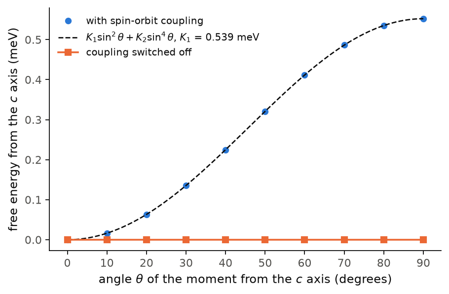
The figure shows cobalt in a tetragonal cell with \(c/a = 1.3\), where the moment turns from the \(c\) axis into the basal plane. With spin-orbit coupling the free energy rises by 0.552 meV, so \(c\) is the easy axis. The curve follows \(K_1\sin^2\theta + K_2\sin^4\theta\) with \(K_1 = 0.539\) meV and a small \(K_2\). With the coupling switched off (soc_scale=0 in the same file) the curve is flat to \(10^{-10}\) meV, which is the check that the anisotropy comes only from the coupling.

Code of this figure (docs/figures/anisotropy_energy_vs_angle/)

compute.py

"""The energy of tetragonal cobalt against the direction of its moment."""
import numpy as np
from defuqumat import Calculator
from common import PSEUDO, save

scalar = Calculator.from_file("co.in", pseudo_dir=PSEUDO)      # no spin-orbit coupling
spinor = Calculator.from_file("co-soc.in", pseudo_dir=PSEUDO)  # with it

angles = np.arange(0, 91, 10)                       # from the c axis towards a
directions = [(np.sin(np.radians(a)), 0.0, np.cos(np.radians(a))) for a in angles]
ry_to_mev = 13605.693
curves = {}
for name, scale in (("soc", 1.0), ("off", 0.0)):    # off: coupling scaled to zero
    mae = scalar.get_anisotropy(spinor, directions=directions, soc_scale=scale)
    curves[name] = (mae.free_energies - mae.free_energies[0]) * ry_to_mev
    curves[name + "_band"] = mae.energies_mev
torque = scalar.get_torque(spinor)                  # the slope at 45 degrees

save(angles=angles, K_torque=torque.anisotropy_constant_mev, **curves)

plot.py

"""The free energy against the angle of the moment, with and without spin-orbit coupling."""
import numpy as np
import style

d = np.load("data.npz")
theta = np.radians(d["angles"])
s2 = np.sin(theta) ** 2
k1, k2 = np.linalg.lstsq(np.stack([s2, s2 ** 2], axis=1), d["soc"], rcond=None)[0]
grid = np.radians(np.linspace(0, 90, 181))


def draw():
    fig, ax = style.figure()
    ax.plot(d["angles"], d["soc"], "o", label="with spin-orbit coupling")
    ax.plot(np.degrees(grid), k1 * np.sin(grid) ** 2 + k2 * np.sin(grid) ** 4,
            **style.reference(),
            label=r"$K_1\sin^2\theta + K_2\sin^4\theta$, $K_1$ = %.3f meV" % k1)
    ax.plot(d["angles"], d["off"], "s-", label="coupling switched off")
    ax.set_xlabel(r"angle $\theta$ of the moment from the $c$ axis (degrees)")
    ax.set_ylabel("free energy from the $c$ axis (meV)")
    ax.set_xticks(d["angles"])
    ax.legend()
    return fig


style.main(draw)

The torque

Let us now get the anisotropy from a single slope. For \(E(\theta) = K\sin^2\theta\) the slope at 45 degrees is \(K\) itself. So one calculation of the slope, the torque, gives the anisotropy constant with no difference of two large numbers. We take the slope of the free energy by automatic differentiation with respect to the direction of the moment:

torque = scalar.get_torque(spinor)          # the slope at 45 degrees
print(f"K = {torque.anisotropy_constant_mev:.4f} meV")

K = 0.5523 meV

The torque gives \(K_1 + K_2 = 0.5523\) meV, the same as the free-energy difference above. get_relaxed_orientation(spinor, rotation=...) follows the torque from a starting orientation, as a relaxation follows the forces. It ends on the easy axis of a ferromagnet, or on the plane of a spiral in a supercell. get_relaxed_anisotropy() takes the other route. It runs a full SCF with spin-orbit coupling for each direction, so the density relaxes too, and the anisotropy is a difference of total energies.

Turning the moment inside the SCF

Here we let the SCF turn the moment itself. A self-consistent run with spin-orbit coupling can in principle turn its own moment. In practice the push on the direction is tiny compared with everything else the SCF balances, and the moment wanders. With rotate_moments=True the code turns the moments along the torque after each step of the SCF. Here the cobalt moment starts 45 degrees away from \(c\):

tilted = Calculator.from_file(folder + "co-tilted.in", pseudo_dir="tests/data/pseudo")
scf = tilted.get_scf(rotate_moments=True, conv_thr=1e-12, torque_conv_thr=1e-9)
m = scf.magnetization_vector
print(f"{scf.iterations} iterations, m = {np.round(m, 4)}")

53 iterations, m = [ 0.     -0.      1.7836]

We see that the moment ends on the \(c\) axis. torque_conv_thr is the threshold on the torque, in Ry per radian.

Limits

The force theorem gives an error for a Hubbard \(U\), because its occupation matrix is not carried from the first run to the second, and for a potential-only meta-GGA, for the same reason with \(\tau\). It also gives an error for a converged magnetic field or constrained moment, because the energy of the field is not in the reported total, and for a spin spiral. A spiral has its own first-order term, on the page about spin spirals. The first run must be spin-polarized, and the second needs noncolin and lspinorb. A direction other than the one in the input needs nosym, because the magnetic symmetry, and with it the k-point set, depends on where the moment points. For get_anisotropy, a first run whose magnetization is genuinely noncollinear gives an error, because the moment is laid along one axis.

A PAW dataset needs the one-file route, meaning the same fully relativistic file for both runs, with soc_scale = 0 for the first. With two different files PAW gives an error, because the one-centre terms are built from the one-centre occupations of the first run, which do not fit the projectors of the other file.

soc_scale outside \([0, 1]\) gives an error on every dataset. For ultrasoft and PAW datasets it must be exactly 0 or 1, because a blend in between is not the overlap of any set of projectors. When every dataset is norm-conserving, any value in \([0, 1]\) is allowed.

get_torque, get_orientation_torque and get_relaxed_orientation give an error for the same cases as the force theorem. get_torque also gives an error for every PAW dataset, because it does not take the one-centre occupations of the first run. get_orientation_torque and get_relaxed_orientation do take PAW on the one-file route. They also take a genuinely noncollinear first run, and turn its texture as it is.

rotate_moments needs a magnetic noncollinear run with spin-orbit coupling, so it gives an error without lspinorb or with soc_scale = 0, where every orientation has the same energy and the step would only follow noise. It also gives an error for a spin spiral, for a Hubbard \(U\), whose occupation matrix would have to turn with the density, and for a magnetic field or a constrained moment, which holds the orientation that the step moves. A run with symmetry needs calc.with_turning_moments() first. This keeps only the identity and the inversion, because only these stay symmetries when all moments turn together, and it builds the k-points again with them. Without it, the run gives an error, because the symmetry of the starting direction would keep the moments in a fixed plane or axis, so the run could not leave it. For a PAW dataset rotate_moments still needs nosym. It does take PAW datasets. On PAW nickel the run stalls with the torque near \(10^{-4}\), and there you should use get_relaxed_orientation instead.

get_relaxed_anisotropy gives an error for a magnetic field or constrained moment, because the energy of the field is not in the total, for a potential-only meta-GGA, which has no energy functional, for a spin spiral and for a collinear run. It needs lspinorb and nosym. Nothing holds the moment while the density relaxes, so the code warns when a direction drifted more than one degree from where it started, and when a direction did not converge. Read converged and drifts on the result before the anisotropy itself.

The notebooks for this page are 36, magnetocrystalline anisotropy and 47, turning a magnet.