Collinear and noncollinear magnetism

In this page we compute magnetic ground states. We start with a collinear magnet with two spin channels, then we compute a noncollinear texture with a moment on each atom, and finally we see how to go from one regime to the other.

Two spin channels

We start with the simplest case, a collinear magnet. With nspin = 2 the density has two parts, \(n_\uparrow\) and \(n_\downarrow\), and the moment is the integral of their difference:

\[ n_\sigma(\mathbf r) = \sum_{n\mathbf k} f_{n\mathbf k\sigma}\, |\psi_{n\mathbf k\sigma}(\mathbf r)|^2, \qquad M = \int \big(n_\uparrow - n_\downarrow\big)\, d\mathbf r . \]

The two channels see different exchange-correlation potentials, \(v_{xc}^\sigma = \delta E_{xc}/\delta n_\sigma\), so the bands of the two channels come out at different energies. This shift is the exchange splitting, and it is the whole of band magnetism. There is one Fermi level for both channels, unless tot_magnetization fixes the moment. starting_magnetization only seeds the first density, with a value between \(-1\) and 1 for each species, and the moment is a result of the SCF. The moment per cell is what a magnetometer measures, and neutron diffraction and XMCD see the moment on each atom. Here we take nickel:

import numpy as np
from defuqumat import Calculator

nickel = Calculator.from_file("docs/figures/magnetism_nickel_dos/ni.in",
                              pseudo_dir="tests/data/pseudo")
scf = nickel.get_scf()
print(f"total energy {scf.total_energy:.8f} Ry")
print(f"magnetization {scf.magnetization:.4f} mu_B per cell")
print(scf.eigenvalues_by_spin.shape)      # (spin, k-points, bands)

total energy -85.72339901 Ry
magnetization 0.7280 mu_B per cell
(2, 10, 9)

scf.magnetization is the moment of the cell in Bohr magnetons. The eigenvalues and the occupations have a first axis for the spin channel in scf.eigenvalues_by_spin and scf.occupations_by_spin. The density scf.density has the shape (2, grid), with the two channels, and get_bands and get_dos also give both channels.

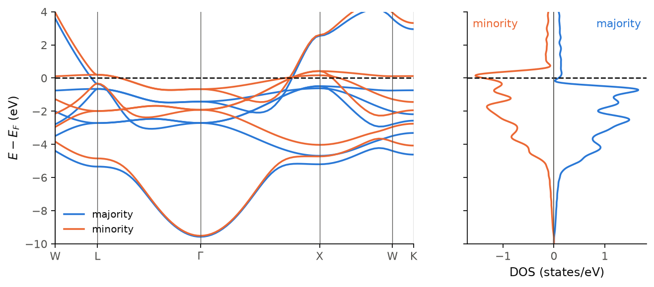
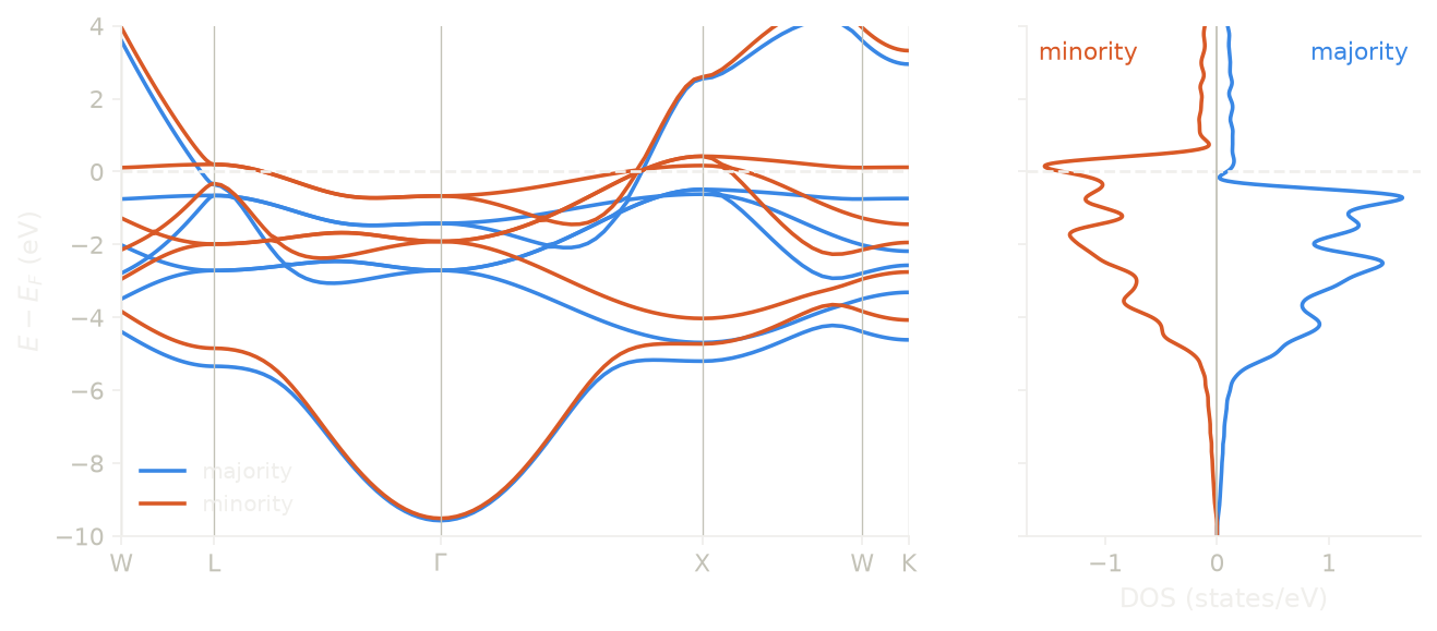
The figure shows fcc nickel in LSDA. We see that the minority \(d\) bands (orange) are the majority \(d\) bands (blue) pushed up by 0.5 to 0.9 eV, for example by 0.80 eV at \(\Gamma\). The majority \(d\) band is full and lies below \(E_F\). The minority \(d\) band crosses \(E_F\), so it has holes, and the number of these holes is the moment, 0.728 \(\mu_B\), against a measured 0.61 \(\mu_B\). This is the Stoner picture of a band magnet. In the DOS on the right, the minority channel is drawn to the left. The broad band that starts at \(-9.6\) eV at \(\Gamma\) is the \(4s\) band. Its exchange splitting there is 0.06 eV, because the moment sits in the \(d\) shell.

Code of this figure (docs/figures/magnetism_nickel_dos/)

compute.py

"""The bands and the DOS of fcc nickel, for each spin channel."""
import numpy as np
from defuqumat import Calculator
from defuqumat.system.kpoints import KPoints
from defuqumat.units import RY_TO_EV
from common import PSEUDO, save

calc = Calculator.from_file("ni.in", pseudo_dir=PSEUDO)
scf = calc.get_scf()
ef = scf.fermi_energy

# W - L - Gamma - X - W - K, in units of 2 pi / a
corners = [[0.5, 0.25, 0.75], [0.5, 0.5, 0.5], [0.0, 0.0, 0.0],
           [0.0, 0.0, 1.0], [0.5, 0.25, 0.75], [0.375, 0.375, 0.75]]
counts = [24, 32, 32, 16, 12, 1]
path = KPoints.band_path(corners, counts, calc.system.cell, crystal=False)
bands = calc.get_bands(kpoints=path, nbnd=9)

dos = calc.get_dos(grid=(16, 16, 16), nbnd=9)
save(x=bands.path_length, bands=(np.asarray(bands.eigenvalues_by_spin) - ef) * RY_TO_EV,
     ticks=bands.path_length[np.cumsum([0] + counts[:-1])],
     energies=(dos.energies - dos.fermi_energy) * RY_TO_EV, dos=dos.dos / RY_TO_EV,
     moment=scf.magnetization)

plot.py

"""The bands and the DOS of nickel: majority and minority channels."""
import numpy as np
import style

d = np.load("data.npz")
labels = ["W", "L", r"$\Gamma$", "X", "W", "K"]


def draw():
    fig, (a, b) = style.figure(2, gridspec_kw={"width_ratios": [2, 1]}, sharey=True)
    for spin, name in enumerate(["majority", "minority"]):
        for n in range(d["bands"].shape[2]):
            a.plot(d["x"], d["bands"][spin, :, n], color=style.color(spin),
                   label=name if n == 0 else None)
        sign = 1 if spin == 0 else -1
        b.plot(sign * d["dos"][spin], d["energies"], color=style.color(spin))
    for t in d["ticks"]:
        a.axvline(t, color=style.ink2(), lw=0.6)
    a.set_xticks(d["ticks"], labels)
    a.set_xlim(d["x"][0], d["x"][-1])
    a.set_ylim(-10.0, 4.0)
    a.set_ylabel(r"$E - E_F$ (eV)")
    a.legend(loc="lower left")
    for ax in (a, b):
        ax.axhline(0.0, **style.reference())
    style.zero_line(b, vertical=True)
    b.set_xlabel("DOS (states/eV)")
    b.text(0.03, 0.97, "minority", transform=b.transAxes, va="top", color=style.color(1))
    b.text(0.97, 0.97, "majority", transform=b.transAxes, va="top", ha="right",
           color=style.color(0))
    return fig


style.main(draw)

Where the moment sits

We now look at the moment in real space. The difference \(n_\uparrow(\mathbf r) - n_\downarrow(\mathbf r)\) is the spin density, which is what polarized neutron diffraction measures. The two channels are in scf.density, so we only subtract them. We also project the moment on the atomic orbitals with get_pdos(), as in the page about the density of states:

m = scf.density[0] - scf.density[1]          # the spin density, mu_B/bohr^3
print(f"{float(m.mean()) * float(nickel.system.cell.volume):.4f} mu_B in the cell")

pdos = nickel.get_pdos()
up, down = pdos.charges.charges_by_spin[:, 0]  # s, p and d of the one atom
print(f"d shell {up[2] - down[2]:.4f} mu_B, s shell {up[0] - down[0]:.4f} mu_B")

0.7280 mu_B in the cell
d shell 0.7396 mu_B, s shell 0.0069 mu_B

The integral of the spin density is the moment of the cell. For an ultrasoft dataset like this one, scf.density already holds the augmentation charge, so nothing is missing from it. The Löwdin moments say that the moment is in the \(d\) shell. Together, the \(d\) and \(s\) shells hold 0.747 \(\mu_B\), more than the 0.728 \(\mu_B\) of the cell, so the part of the density that the atomic orbitals do not describe carries a small negative moment, \(-0.019\,\mu_B\).

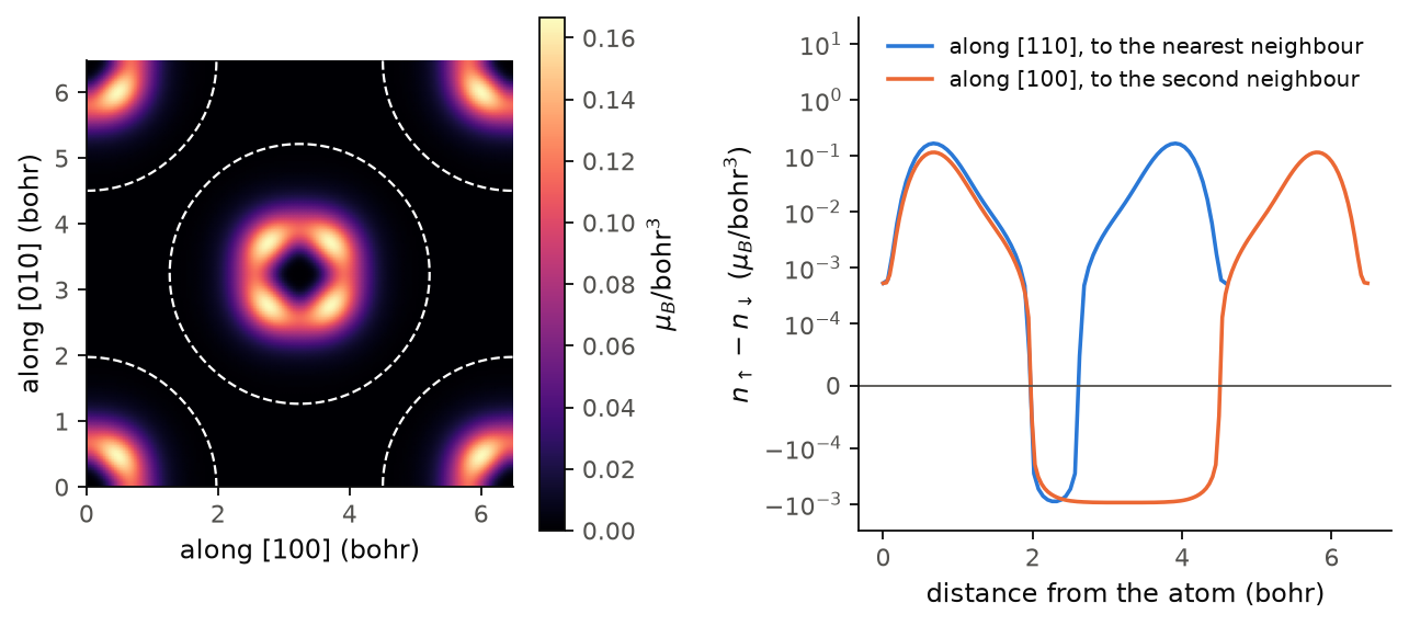
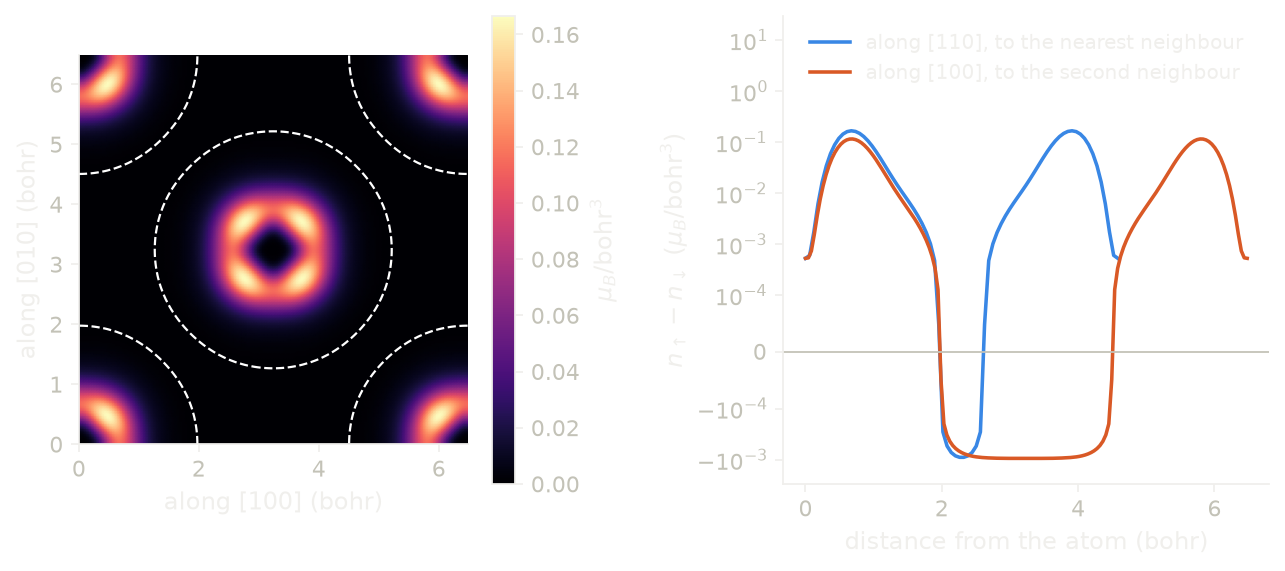
The left panel shows the spin density on the (001) face of the cubic cell, with an atom at each corner and one in the centre. Around each atom the spin density is a ring at about 0.7 bohr from the nucleus, the radius of the \(3d\) shell, and it is close to zero at the nucleus, as for a \(d\) orbital. The ring is not round. Its maxima point along [110], towards the nearest neighbours, where it reaches 0.167 \(\mu_B\)/bohr\(^3\), while along [100] it reaches 0.115 \(\mu_B\)/bohr\(^3\). So the moment sits more in the \(t_{2g}\) orbitals, which point between the cubic axes, than in the \(e_g\) orbitals, which point along them. Polarized neutron diffraction on nickel also finds most of the \(3d\) moment in the \(t_{2g}\) orbitals. The white dashed line is where the spin density changes sign. Between the atoms it is negative, about \(-1\times10^{-3}\,\mu_B\)/bohr\(^3\), as the right panel shows on a logarithmic scale. These are the electrons between the atoms, polarized opposite to the \(d\) shell, and their sign and size agree with the \(-0.019\,\mu_B\) of the Löwdin balance above. These small numbers come from the \(4\times4\times4\) mesh of the SCF, and we did not converge them in the k-mesh.

Code of this figure (docs/figures/magnetism_spin_density/)

compute.py

"""The spin density of nickel on a face of the cubic cell, and the moment of each orbital."""
import numpy as np
from defuqumat import Calculator
from common import PSEUDO, save

nickel = Calculator.from_file("ni.in", pseudo_dir=PSEUDO)
scf = nickel.get_scf()
n = np.asarray(scf.density)                  # (up, down) on the FFT grid, 1/bohr^3
m = n[0] - n[1]                              # the spin density, mu_B/bohr^3
omega = float(nickel.system.cell.volume)
print(f"moment: {m.mean() * omega:.4f} from the grid, {scf.magnetization:.4f} from the SCF")

# the Fourier coefficients: m(r) = sum_G c_G exp(i G.r), the small ones dropped
c = np.fft.fftn(m).ravel() / m.size
grid = np.meshgrid(*[np.fft.fftfreq(k) * k for k in m.shape], indexing="ij")
g = np.stack([x.ravel() for x in grid], axis=1) @ np.asarray(nickel.system.cell.bg)
keep = abs(c) > 1e-7 * abs(c).max()
c, g = c[keep], g[keep]

# the (001) face of the cubic cell, z = 0, with atoms at the corners and the centre
alat = nickel.system.cell.alat
s = np.linspace(0.0, alat, 151)
image = np.array([(np.exp(1j * (x * g[:, 0] + s[:, None] * g[:, 1])) @ c).real
                  for x in s])

# the Lowdin moment of each orbital, majority minus minority
pdos = nickel.get_pdos()
charges = pdos.charges.charges_by_spin[:, 0]  # (spin, l) on the one atom
print("Lowdin moments s, p, d:", charges[0] - charges[1], "spilling", pdos.charges.spilling)
save(s=s, spin_density=image, orbital_moment=charges[0] - charges[1],
     moment=scf.magnetization, grid_moment=m.mean() * omega)

plot.py

"""The spin density of nickel on the (001) face of the cubic cell, and two cuts through it."""
import numpy as np
import style

d = np.load("data.npz")
s, m = d["s"], d["spin_density"]


def draw():
    fig, (a, b) = style.figure(2, gridspec_kw={"wspace": 0.45})
    mesh = a.pcolormesh(s, s, m.T, shading="gouraud", vmin=0.0)
    a.contour(s, s, m.T, levels=[0.0], colors="white", linestyles="--", linewidths=1.0)
    a.set_aspect("equal")
    a.set_xlabel("along [100] (bohr)")
    a.set_ylabel("along [010] (bohr)")
    style.colorbar(fig, mesh, a, r"$\mu_B$/bohr$^3$")

    # from the atom at the corner to the next atom, along [110] and along [100]
    n = len(s)
    b.plot(np.sqrt(2) * s[: n // 2 + 1], np.diag(m)[: n // 2 + 1], color=style.color(0),
           label="along [110], to the nearest neighbour")
    b.plot(s, m[:, 0], color=style.color(1), label="along [100], to the second neighbour")
    style.zero_line(b)
    b.set_yscale("symlog", linthresh=1e-4)
    b.set_ylim(-3e-3, 30.0)
    b.set_xlabel("distance from the atom (bohr)")
    b.set_ylabel(r"$n_\uparrow - n_\downarrow$ ($\mu_B$/bohr$^3$)")
    b.legend(loc="upper center")
    return fig


style.main(draw)

Noncollinear magnetism

We now let the moments point in any direction. With noncolin = .true. the wavefunctions are two-component spinors, and the magnetization is a vector field:

\[ \mathbf m(\mathbf r) = \sum_{n\mathbf k} f_{n\mathbf k}\, \psi^{\dagger}_{n\mathbf k}(\mathbf r)\,\boldsymbol\sigma\,\psi_{n\mathbf k}(\mathbf r) . \]

Without spin-orbit coupling the energy does not depend on the direction of all moments together, only on their angles to each other. We give the direction of the starting moment of a species with angle1 (from \(z\)) and angle2 (from \(x\)), as in pw.x. To give each atom its own direction, you add a STARTING_MOMENTS card with one row \((m_x, m_y, m_z)\) per atom. Here we take four hydrogen atoms in a chain, with moments 90 degrees apart in the plane across the chain:

helix = Calculator.from_file("docs/figures/magnetism_texture/h4-helix.in",
                             pseudo_dir="tests/data/pseudo")
scf = helix.get_scf()
print(np.round(scf.site_moments, 4))      # mu_B, one row per atom
print(f"cell: {np.round(scf.magnetization_vector, 5)}")

[[ 0.4681  0.      0.    ]
 [ 0.      0.4681 -0.    ]
 [-0.4681 -0.     -0.    ]
 [ 0.     -0.4681  0.    ]]
cell: [ 0. -0. -0.]

scf.site_moments is the moment in a sphere around each atom, one row per atom, in \(\mu_B\), and scf.site_charges is the charge in the same spheres. We see that the moment of the cell is zero, because the four moments cancel. An antiferromagnet and a cell with no moment at all give the same zero, so for a compensated magnet you have to look at the site moments. The code takes the radius of the spheres a little under half the distance to the nearest neighbour, divided by 1.2 for the tapered edge, so that the spheres do not overlap. This radius is a choice, so you should compare site moments with another code only at the same radius.

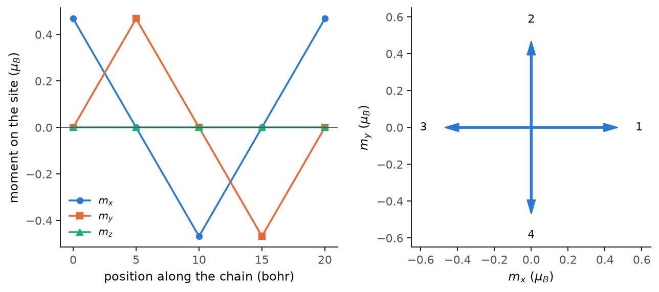
The left panel shows the three components of the moment on each site along the chain. The point at 20 bohr is the first atom of the next cell, so the turn closes. The right panel shows the four moments seen along the chain. They are 0.468 \(\mu_B\) each and exactly 90 degrees apart, and \(m_z\) is zero. The code keeps only the symmetry operations that map this texture onto itself, four of them here, so the texture is not averaged away during the SCF.

Code of this figure (docs/figures/magnetism_texture/)

compute.py

"""A 90-degree helix on a hydrogen chain: the moment on each site."""
import numpy as np
from defuqumat import Calculator
from common import PSEUDO, save

calc = Calculator.from_file("h4-helix.in", pseudo_dir=PSEUDO)
scf = calc.get_scf()
z = np.asarray(calc.system.structure.positions)[:, 2]        # bohr

save(z=z, moments=np.array(scf.site_moments),
     cell_moment=np.array(scf.magnetization_vector), length=float(calc.system.cell.at[2, 2]))

plot.py

"""The moments of the helix along the chain, and seen along the chain."""
import numpy as np
import style

d = np.load("data.npz")
m = np.vstack([d["moments"], d["moments"][:1]])          # close the turn
z = np.append(d["z"], d["z"][0] + d["length"])


def draw():
    fig, (a, b) = style.figure(2)
    a.plot(z, m[:, 0], "o-", label="$m_x$")
    a.plot(z, m[:, 1], "s-", label="$m_y$")
    a.plot(z, m[:, 2], "^-", label="$m_z$")
    style.zero_line(a)
    a.set_xlabel("position along the chain (bohr)")
    a.set_ylabel(r"moment on the site ($\mu_B$)")
    a.legend()
    for site, (mx, my, _) in enumerate(d["moments"]):
        b.annotate("", xy=(mx, my), xytext=(0, 0),
                   arrowprops=dict(width=1.4, headwidth=7, color=style.color(0)))
        b.text(1.25 * mx, 1.25 * my, str(site + 1), ha="center", va="center")
    b.set_xlim(-0.65, 0.65)
    b.set_ylim(-0.65, 0.65)
    b.set_aspect("equal")
    b.set_xlabel(r"$m_x$ ($\mu_B$)")
    b.set_ylabel(r"$m_y$ ($\mu_B$)")
    return fig


style.main(draw)

Let us now start the same chain from another texture. with_moments gives a new calculator with another set of starting moments, with no new input file, and the new run starts from these moments and not from the old density:

afm = helix.with_moments([[0, 0, 0.6], [0, 0, -0.6]] * 2)
scf = afm.get_scf()
print(np.round(scf.site_moments, 4))
print(f"energy against the helix {scf.total_energy - helix.get_scf().total_energy:+.6f} Ry")

[[-0.      0.      0.6007]
 [ 0.     -0.     -0.6007]
 [ 0.     -0.      0.6007]
 [-0.     -0.     -0.6007]]
energy against the helix -0.008368 Ry

The collinear antiferromagnet is 8.4 mRy below the helix, so the helix is not the ground state of this chain. Nothing in the SCF turns a moment towards a lower texture. A run converges to a state close to where it starts, and it reports convergence just as well. So when you look for the ground state, you should compare several starting textures.

Holding a moment: constraints and fields

We now hold a moment in place. To compute a state that is not a minimum, for example two moments at a fixed angle, we hold the moment with a constraint. constrained_magnetization in &system chooses what is held, as in pw.x: 'total' (the moment of the cell), 'atomic' (the moment of each atom), 'atomic direction' (only its direction) and 'total direction'. With 'atomic texture' each atom keeps the direction of its row in a STARTING_MOMENTS card. Each adds a penalty with the weight lambda:

\[ E_{\rm pen} = \lambda \sum_I \big(\mathbf m_I - \mathbf m^{\rm fix}_I\big)^2 . \]

A penalty still pushes at convergence, so the moment ends a bit away from its target. 'atomic fsm' instead adjusts a field on each atom until the moment is exactly at its target, as in Elk. 'fsm' does this for the moment of the cell, and 'atomic fsm direction' does the same for the direction only. The field that does this is then a result, and it is the torque that the texture costs. How far each atom is from its target is in scf.site_residuals, one number per atom, in degrees for a direction and in \(\mu_B\) for a moment. For a fixed external field you use the B_field of pw.x, or a field on each atom with a LOCAL_MAGNETIC_FIELDS card. The energy of a penalty or of a field is not part of the total energy, and the code prints it apart, as in pw.x and Elk.

From one spin regime to another

Here we start a run in one spin regime from a converged run in another. This goes from unpolarized to collinear, from collinear to noncollinear, or to a fully relativistic dataset with spin-orbit coupling. with_spin(nspin) returns a new calculator whose SCF starts from the converged density of the old one. Here we take the nickel run above to spinors:

spinor = nickel.with_spin(4)              # noncollinear, from the collinear state
scf = spinor.get_scf()
print(f"{scf.iterations} iterations, m = {np.round(scf.magnetization_vector, 4)}")

1 iterations, m = [ 0.    -0.     0.728]

The noncollinear run starts at the converged collinear density, so it needs one iteration. This is how a magnetic anisotropy calculation starts in practice, as we see in the page about anisotropy. From an unpolarized run to a collinear one, the code seeds the moment, because nothing in the SCF breaks the spin symmetry by itself. Without a seed, the run would stay unpolarized and still report convergence.

The argument magnetization of with_spin and with_moments says how the moment of the old run crosses into the new one. 'auto', the default of with_spin, carries the old moment where there is one and seeds starting_magnetization where there is none. 'seed', the default of with_moments, keeps the converged charge and takes the moment from the new starting moments. 'carry' always carries the old moment, and 'none' starts unpolarized.

The source-free exchange-correlation field

Let us now ask what turns a moment. A local functional builds the exchange-correlation field \(\mathbf B_{xc}(\mathbf r)\) along \(\mathbf m(\mathbf r)\) at every point, so the torque \(\boldsymbol\tau = \int \mathbf m\times\mathbf B_{xc}\, d\mathbf r\) is zero at every density, converged or not. A magnetic field in nature has no sources, and nosource = .true. in &system makes the exchange-correlation field obey that, as in Elk. We remove the longitudinal part of \(\mathbf B_{xc}\), the part with a divergence, and the field is then no longer parallel to \(\mathbf m\). We compute the torque with calc.get_exchange_torque(). Its sites hold one torque vector per atom, and its parallel_fraction is 1 without nosource, so that a zero torque can be told from a field that is parallel to the moment by construction. Without spin-orbit coupling the total torque of the cell is zero by symmetry, so what we read is the torque on each site.

Limits

With occupations = 'fixed' and two spin channels, you must give tot_magnetization, and it must be an integer, as in pw.x. tot_magnetization with any nspin other than 2 gives an error, as in pw.x. A noncollinear run holds its total moment with constrained_magnetization = 'total' instead. An SCF or a relaxation with nspin = 2 and no starting_magnetization gives an error, as in pw.x, because nothing in the SCF breaks the spin symmetry by itself and the run would converge to the unpolarized state. An explicit starting_magnetization = 0.0 is accepted, and so is a run with tot_magnetization, with a constraint or with occupations = 'from_input'.

noncolin with angle1 or angle2 and no starting_magnetization gives an error, because the angles then give the direction of a moment that has no length. A spinor run with no magnetization at all is still allowed. STARTING_MOMENTS needs noncolin for any \(x\) or \(y\) component, and it needs one row per atom.

'total', 'total direction', 'atomic direction' and 'atomic texture' need noncolin = .true., so 'total direction' or 'atomic direction' with nspin = 2 gives an error, as in pw.x. 'atomic' and 'atomic direction' need some starting_magnetization or a STARTING_MOMENTS card, because the targets are built from them and would all be zero otherwise. 'atomic texture' needs a STARTING_MOMENTS card with no zero row, because a zero vector has no direction. The code also warns that 'atomic texture' did not converge at any lambda we tried, so for a texture you use 'atomic' with the same card, scaled to the moment you expect.

The field schemes 'fsm', 'atomic fsm' and 'atomic fsm direction' together with lspinorb = .true. give an error, because the search updates each Cartesian component of the field from the same component of the moment, and spin-orbit coupling couples the components. So there you use 'total' or 'atomic'. These three schemes with reducebf below 1 also give an error. The Newton solver (scf_solver = 'newton-krylov') runs with these three schemes, with the limits listed on the ground-state page. On a canted pair it needs about 60 steps, so give it scf_solver_options={"max_iterations": 80}. 'atomic fsm' and 'atomic fsm direction' need noncolin = .true. and a STARTING_MOMENTS card, and they cannot be used together with a LOCAL_MAGNETIC_FIELDS card. 'atomic fsm direction' gives an error for a zero row in the card. With these two schemes and fsm_update = 'elk', the default, the code warns unless mixing_mode = 'adaptive', because the other mixers run away. mixing_mode = 'adaptive' with mixing_beta = 0.05 is what Elk uses.

In a collinear run, a symmetry operation that reverses every moment is a symmetry only when combined with time reversal. The code drops these operations, as pw.x does with colin_mag = 1, which gives the same result at the cost of more k-points. The symmetry group comes from the input and not from the density, so a texture that you pass only in starting_density is averaged away. The code warns when symmetrization changes such a starting density by more than \(10^{-3}\) of its size. Give the texture as a STARTING_MOMENTS card, or set nosym = .true..

The site moments are the moments in spheres that do not overlap, with a radius a little under half the distance to the nearest neighbour, divided by 1.2. So the site charges and the site moments sum to less than those of the cell. The SCF and the relaxations report them, and the response calculations do not.

A collinear source cannot be promoted to a target whose atoms point along different axes, from angle1 and angle2 or from a STARTING_MOMENTS card, because one scalar magnetization cannot follow a helix. A noncollinear magnetization that does not lie along one axis cannot be split back into two collinear channels. In both cases magnetization='seed' keeps the converged charge and takes the moment from the new starting moments. magnetization='carry' gives an error when the source has no moment. A spiral measures \(m_x\) and \(m_y\) in the frame that turns with \(\mathbf q\). So a noncollinear magnetization crosses into a spiral, or out of one, only when \(\mathbf q\) is a reciprocal lattice vector of the cell, for example spiral_q = (0, 0, 1) or zero. Then the code turns \(m_x\) and \(m_y\) by the angle \(\mathbf q\cdot\mathbf r\), and the new run starts on its fixed point. For any other \(\mathbf q\) the spiral repeats only in a supercell, so it gives an error. A DFT+U state does not cross this boundary. A collinear source does cross, and a spiral continues from another spiral at any \(\mathbf q\). A spiral does not continue into a collinear run (nspin = 2), because its moment turns from point to point. The kinetic energy density of a meta-GGA run does not cross this boundary, so the new run builds its own.

The source of a continuation must have the same cell, the same grid and the same number of electrons, so a dataset with another z_valence gives an error. The code warns when the source was held by a field or a constraint that the new run does not have, because the moment it carries is then the moment of the field. A value of magnetization other than 'auto' gives an error on a run that continues nothing, on a resume from a checkpoint, which continues the same run, and beside a continued state that already says how the moment crosses.

A spin spiral whose starting moments all lie along \(z\), or are all zero, gives an error, also at \(\mathbf q = 0\). The spiral turns the moments about \(z\), so such a run would converge to the ferromagnet at every \(\mathbf q\). angle1 = 90 puts the moments in the plane.

nosource gives an error for forces, stress, phonons, the elastic constants and all the linear response, because the projection changes the potential and not the energy. For the same reason the code warns that the total energy of a nosource run cannot be compared with that of a run without it. The magnons give an error, because their kernel \(B_{xc}/m\) is a scalar only while \(\mathbf B_{xc}\) is parallel to \(\mathbf m\). nosource also gives an error in a collinear run, with a PAW dataset, on a spin spiral, with a potential-only meta-GGA, with noncollinear_gga = 'grad_m' asked for explicitly and in the ultracell. If you do not give noncollinear_gga, a nosource run uses 'kubler'. Elk calls nosource an experimental feature, and this holds here too. The scaling of the spin part of the field, the other option of Elk, is not implemented.

The noncollinear linear response gives an error.

The notebooks for this page are 07, spin polarization, 11, noncollinear magnetism and fields, 43, magnetic textures and 18, continuing a calculation.