Real-time evolution
On this page we evolve a state in real time,
\(|\psi(t)\rangle=e^{-iHt}|\psi(0)\rangle\), and measure an observable along
the way. The typical case is a quantum quench: we prepare the ground state
of a Hamiltonian \(H_0\), change the Hamiltonian to \(H_1\) at \(t=0\), and follow
how observables oscillate, relax or thermalize. Here h0 and h1 are two
Hamiltonians of the chain sc, for example a staggered field and the
Heisenberg chain of Ground state.
from dmrgpy import timedependent
sc.set_hamiltonian(h0)
wf0 = sc.get_gs()                          # ground state of H0
sc.set_hamiltonian(h1)                     # quench to H1
(ts, sz) = timedependent.evolve_and_measure(sc, operator=sc.Sz[0],
                                            nt=200, dt=0.02, wf=wf0)
This gives \(\langle\psi(t)|S^z_0|\psi(t)\rangle\) at the times \(t=0,\,dt,\,2dt,\dots\). The keywords are:
nt,dt: the number of time steps (default 1000) and the time step (default 0.01). A smallerdtis more accurate.wf: the initial state. Without it, the ground state of the chain is used.h: the Hamiltonian of the evolution, if not the one of the chain.mode="ED": exact evolution, the reference for small chains.return_wf=True(DMRG): also return the final state as a third output.
The accuracy of the DMRG evolution is set by sc.maxm and dt. The
entanglement grows with time after a quench, so the bond dimension needed
grows too. When the result stops agreeing with a larger maxm, the
simulation has reached its maximum time.
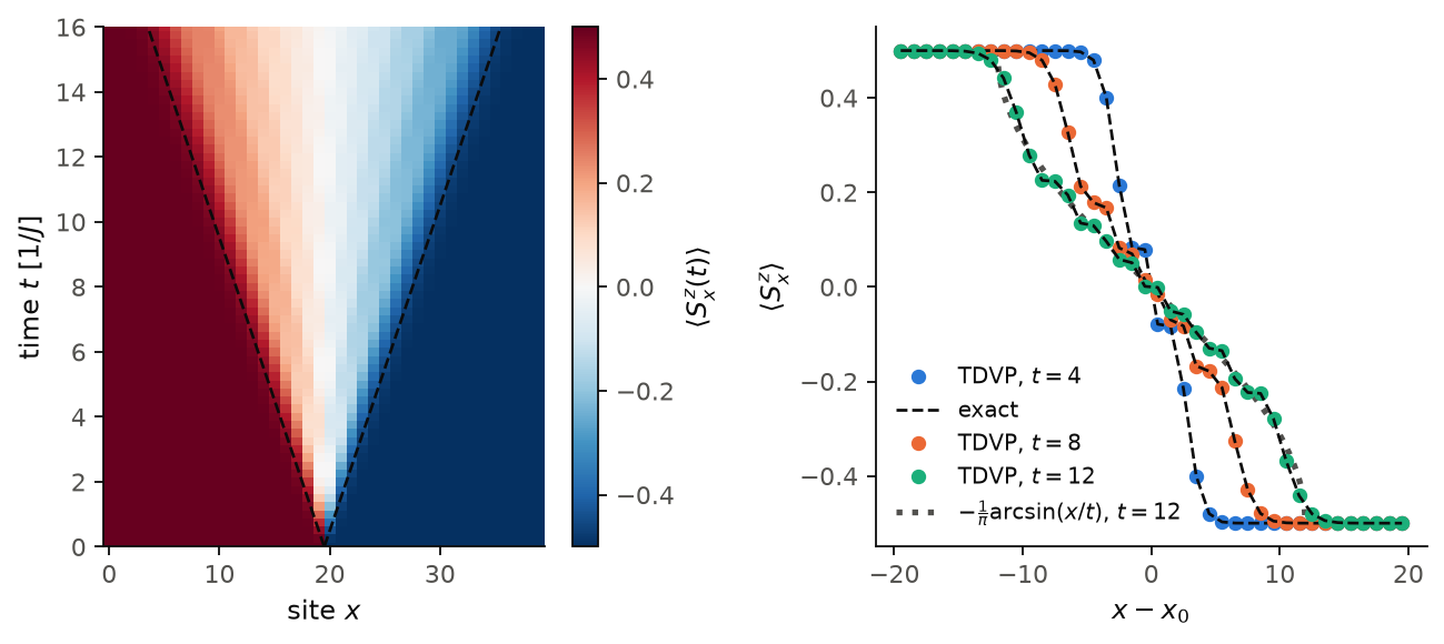
The figure shows a quench in the XX chain, \(H=\sum_i(S^x_iS^x_{i+1}+S^y_iS^y_{i+1})\), with \(n=40\). The initial state is a domain wall, all spins up on the left half and all down on the right half. Left: \(\langle S^z_x(t)\rangle\) from TDVP. The magnetization moves only inside a cone of slope one (dashed lines), since the fastest excitations have velocity \(v=J\). Right: the profile at three times. The model maps to free fermions, so the exact profile is known (dashed lines). TDVP agrees with it to \(10^{-4}\). At long times the profile approaches \(-\frac1\pi\arcsin(x/t)\) (dotted line).
Code of this figure (docs/figures/real-time_light_cone/)
# A domain wall of the spin-1/2 XX chain released at t=0, evolved with TDVP,
# against the exact result: the XX chain is free fermions with hopping 1/2,
# so <Sz_i>(t) = C_ii(t) - 1/2 with C(t) = U C(0) U^dagger, U = exp(-i h t).
import numpy as np
import scipy.linalg
from dmrgpy import spinchain, timedependent

n = 40
dt, nt, nchunks = 0.05, 5, 64  # the profile is stored every nt*dt

sc = spinchain.Spin_Chain(["S=1/2"]*n)
sc.maxm, sc.tevol_method = 100, "TDVP"
# initial state: all up on the left half, all down on the right half
eps = np.where(np.arange(n) < n//2, 1.0, -1.0)
sc.set_hamiltonian(sum(-eps[i]*sc.Sz[i] for i in range(n)))
wf = sc.get_gs()
sc.set_hamiltonian(sum(sc.Sx[i]*sc.Sx[i+1] + sc.Sy[i]*sc.Sy[i+1]
                       for i in range(n-1)))


def profile(wf):
    return [sc.aMb(wf, sc.Sz[i], wf).real for i in range(n)]


sz = [profile(wf)]
for _ in range(nchunks):
    _, _, wf = timedependent.evolve_and_measure(sc, operator=sc.Sz[n//2], nt=nt,
                                                dt=dt, wf=wf, return_wf=True)
    sz.append(profile(wf))
ts = nt*dt*np.arange(nchunks + 1)

h = 0.5*(np.eye(n, k=1) + np.eye(n, k=-1))
c0 = np.diag((eps > 0).astype(float))
U = [scipy.linalg.expm(-1j*h*t) for t in ts]
sz_exact = [np.real(np.diag(u @ c0 @ u.conj().T)) - 0.5 for u in U]

np.savez("data.npz", n=n, ts=ts, sz=sz, sz_exact=sz_exact)
import numpy as np
import style

d = np.load("data.npz")
n, ts, sz, sz_ex = int(d["n"]), d["ts"], d["sz"], d["sz_exact"]
x0 = n/2 - 0.5  # the wall, between sites n/2-1 and n/2
x = np.arange(n)
dt_row = ts[1] - ts[0]


def draw(theme):
    c = style.colors(theme)
    fig, (ax1, ax2) = style.figure(2)
    # signed quantity: diverging map, dark cone lines on its white middle
    im = ax1.imshow(sz, origin="lower", aspect="auto", cmap="RdBu_r",
                    vmin=-0.5, vmax=0.5,
                    extent=[-0.5, n - 0.5, ts[0] - dt_row/2, ts[-1] + dt_row/2])
    tt = np.linspace(0, ts[-1], 50)
    for s in (+1, -1):
        ax1.plot(x0 + s*tt, tt, color="#0b0b0b", ls="--", lw=style.LW_REF)
    ax1.set_xlim(-0.5, n - 0.5)
    ax1.set_ylim(0, ts[-1])
    ax1.set_xlabel(r"site $x$")
    ax1.set_ylabel(r"time $t$ [$1/J$]")
    style.colorbar(fig, im, ax1, r"$\langle S^z_x(t)\rangle$", theme)

    for j, t in enumerate((4.0, 8.0, 12.0)):
        k = int(np.argmin(np.abs(ts - t)))
        ax2.plot(x - x0, sz[k], "o", color=c["series"][j], ms=style.MS,
                 label=r"TDVP, $t=%g$" % t)
        ax2.plot(x - x0, sz_ex[k], **style.reference(theme),
                 label="exact" if j == 0 else None)
    u = np.linspace(-12.0, 12.0, 200)
    ax2.plot(u, -np.arcsin(u/12.0)/np.pi, color=c["ink2"], ls=":", lw=2.4,
             zorder=0, label=r"$-\frac{1}{\pi}\arcsin(x/t)$, $t=12$")
    ax2.set_xlabel(r"$x-x_0$")
    ax2.set_ylabel(r"$\langle S^z_x\rangle$")
    ax2.legend(loc="lower left")
    fig.subplots_adjust(wspace=0.4)
    return fig


style.main(draw, "real-time_light_cone")
Local quench
evolution_ABA first applies an operator \(A\) to the
state, for example a spin flip or an added electron, and then measures \(B\):
Here we flip up the spin at the edge of the Heisenberg chain and follow how the magnetization arrives at site 3:
Sp0 = sc.Sx[0] + 1j*sc.Sy[0]               # S^+ on site 0
(ts, sz3) = timedependent.evolution_ABA(sc, A=Sp0, B=sc.Sz[3], nt=200, dt=0.02)
It takes the same keywords as evolve_and_measure, and starts from the
ground state of the chain unless wf is given. Note that \(A\) is applied as
it is, so the state \(A|\psi\rangle\) is not normalized.
Evolved states
To get the states themselves, sc.exponential(-1j*t*h,
wf) returns \(e^{-iHt}|\psi\rangle\) for one time (Hamiltonians and operators), and
timeevolution.evolve_WF(h, wf, ts=ts) returns a list of states, one for
each time in ts. Note that evolve_WF applies \(e^{+iht}\), so pass -h
for the physical evolution. With the states, we compute any overlap, for
example the return amplitude \(\langle\psi(0)|\psi(t)\rangle\).
Choosing the propagator
sc.tevol_method selects the algorithm:
"TDVP"(default): two-site TDVP. It works for any Hamiltonian and grows the bond dimension as needed. Onitensor_version=2it is replaced by"MPO"."TDVP_GSE": one-site TDVP with global subspace expansion (Yang and White, PRB 102, 094315 (2020)). Use it when the initial state has a small bond dimension, for example a product state. The bond dimension grows only during the firstsc.tdvp_gse_sweepssteps (default 3); the other settings aresc.tdvp_gse_krylov_order(default 3) andsc.tdvp_gse_cutoff(default \(10^{-8}\))."TDVP_CBE": one-site TDVP with controlled bond expansion (Li, Gleis and von Delft, arXiv:2208.10972). Before each local step, the bond gets the few new states on which \(H|\psi\rangle\) has weight outside the current bond space, and after it the bond is cut back tosc.maxm. Like"TDVP_GSE"it starts well from a product state, but the bond keeps growing at every step, so it follows a quench whose entanglement grows for a long time. Its accuracy is the one of"TDVP".sc.cbe_delta(default 0.1) sets how far a bond is expanded, to \((1+\delta)\)maxmstates. Only onitensor_version="python", 3 and"julia_live"; the other backends raise an error. Seeexamples/time_evolution/tdvp_cbe_VS_ED_time_evolution."TEBD": second-order Trotter evolution with two-site gates. Faster than TDVP, but only for nearest-neighbor Hamiltonians; otherwise it raises an error. ASpinful_Fermionic_Chain_NativeHubbard chain is nearest-neighbor, the interleavedSpinful_Fermionic_Chainis not."AUTO":"TEBD"when the Hamiltonian is nearest-neighbor,"TDVP"otherwise."MPO": a second-order Taylor expansion of \(e^{-iH\,dt}\) applied as an MPO. The only option onitensor_version=2, and less accurate than TDVP at the same bond dimension.
sc.tevol_method = "TEBD"
The same propagator is used by the "TD" and "TDZ" dynamical
correlators (Choosing a correlator method). See examples/time_evolution/time_evolution_quench.