Ground state
On this page we compute the ground state of a chain and measure it. All the examples use a spin-1/2 Heisenberg chain:
from dmrgpy import spinchain
n = 20
sc = spinchain.Spin_Chain(["S=1/2" for i in range(n)])
h = sum(sc.Sx[i]*sc.Sx[i+1] + sc.Sy[i]*sc.Sy[i+1] + sc.Sz[i]*sc.Sz[i+1]
        for i in range(n-1))
sc.set_hamiltonian(h)
Ground-state energy
The ground state is the state with the lowest energy,
e0 = sc.gs_energy()   # E0
wf = sc.get_gs()      # the ground state |GS> as an MPS
DMRG finds this minimum within matrix product states of bond dimension
sc.maxm. The result is exact when maxm is large enough, and an upper
bound on \(E_0\) otherwise. The keywords that control accuracy are:
sc.maxm: the bond dimension. Increase it until \(E_0\) stops changing. Gapped chains need a smallmaxm; critical chains and wide ladders need a large one.sc.nsweeps: the number of DMRG sweeps.sc.dmrg_method = "CBE": one-site updates with bond expansion, cheaper for a large local dimension (One-site updates with bond expansion).gs_energy(maxde=1e-4): doublesmaxmuntil the energy fluctuation per site (Energy fluctuation) is smaller thanmaxde.mode="ED": exact diagonalization, for small chains and for checking DMRG.
The chain stores the ground state. A second call to gs_energy() returns
it without solving again. The sweep schedule and warm starts are on
Controlling the solver.
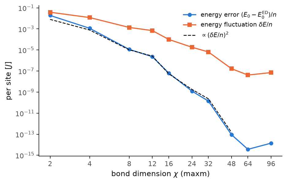
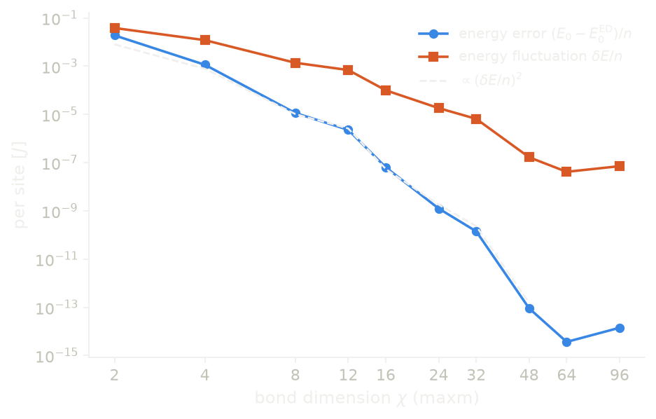
The figure shows the energy error and the energy fluctuation per site of
a Heisenberg chain with \(n=16\), as a function of maxm. The reference is
ED. Both fall fast with maxm. The energy error follows \(\delta E^2\)
(dashed line). From maxm=64 on, both stay at the numerical precision.
Code of this figure (docs/figures/ground-state_convergence/)
# Energy error and energy fluctuation of the spin-1/2 Heisenberg chain
# against the bond dimension, with exact diagonalization as the reference.
import numpy as np
from dmrgpy import spinchain

n = 16
maxms = [2, 4, 8, 12, 16, 24, 32, 48, 64, 96]


def heisenberg():
    sc = spinchain.Spin_Chain(["S=1/2"]*n)
    h = sum(sc.Sx[i]*sc.Sx[i+1] + sc.Sy[i]*sc.Sy[i+1] + sc.Sz[i]*sc.Sz[i+1]
            for i in range(n-1))
    sc.set_hamiltonian(h)
    return sc


e_ed = heisenberg().gs_energy(mode="ED")
energy, de = [], []
for maxm in maxms:
    sc = heisenberg()  # a fresh chain for each bond dimension
    sc.maxm, sc.nsweeps, sc.cutoff = maxm, 20, 1e-14
    energy.append(sc.gs_energy())
    de.append(sc.gs_energy_fluctuation())

np.savez("data.npz", n=n, maxm=maxms, energy=energy, de=de, e_ed=e_ed)
import numpy as np
import style

d = np.load("data.npz")
maxm = d["maxm"]
err = np.abs(d["energy"] - d["e_ed"])/d["n"]  # abs: at the floor it can be < 0
de = d["de"]/d["n"]
# err = c dE^2, c fitted on the points above the numerical floor
fit = err > 5e-14
c_fit = np.exp(np.mean(np.log(err[fit]) - np.log(de[fit]**2)))


def draw(theme):
    c = style.colors(theme)
    fig, ax = style.figure(1)
    ax.plot(maxm, err, "o-", color=c["series"][0],
            label=r"energy error $(E_0-E_0^{\rm ED})/n$")
    ax.plot(maxm, de, "s-", color=c["series"][1],
            label=r"energy fluctuation $\delta E/n$")
    ax.plot(maxm[fit], c_fit*de[fit]**2, **style.reference(theme),
            label=r"$\propto(\delta E/n)^2$")
    ax.set_xscale("log")
    ax.set_yscale("log")
    ax.set_xticks(maxm)
    ax.set_xticklabels([str(m) for m in maxm])
    ax.minorticks_off()
    ax.set_xlabel(r"bond dimension $\chi$ (maxm)")
    ax.set_ylabel(r"per site [$J$]")
    ax.legend()
    return fig


style.main(draw, "ground-state_convergence")
Expectation values
For any operator \(O\) built from the chain operators, as \(H\) is,
mz = [sc.vev(sc.Sz[i]).real for i in range(n)]   # magnetization profile
e2 = sc.vev(h, npow=2)                           # <H^2>
Common profiles have their own methods, each returning one value per site:
get_density(): the occupation \(\langle n_i\rangle\), summed over spin. Fermionic chains.get_density_fluctuation(): \(\langle n_i^2\rangle-\langle n_i\rangle^2\). Fermionic chains.get_onsite_pairing(): \(\langle c_{i\uparrow}c_{i\downarrow}\rangle\). Spinful fermionic chains.get_magnetization(): \(\langle S^x_i\rangle\), \(\langle S^y_i\rangle\), \(\langle S^z_i\rangle\). A \(3\times n\) array on spin chains, and an \(n\times 3\) array on spinful fermionic chains.
Static correlators
A two-point correlator is the expectation value of a product of two operators:
czz = [sc.vev(sc.Sz[0]*sc.Sz[i]).real for i in range(n)]       # <Sz_0 Sz_i>
cdc = fc.vev(fc.Cdag[0]*fc.C[5])   # <c^dag_0 c_5> on a fermionic chain fc
The equal-time structure factor is its Fourier transform, \(S(q)=\sum_{i,j}e^{iq(i-j)}\langle O_iO_j\rangle\). This is the quantity measured by neutron or X-ray diffraction, and it is the frequency integral of the dynamical correlators.
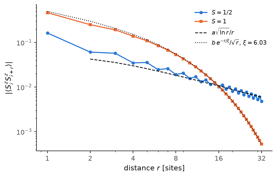
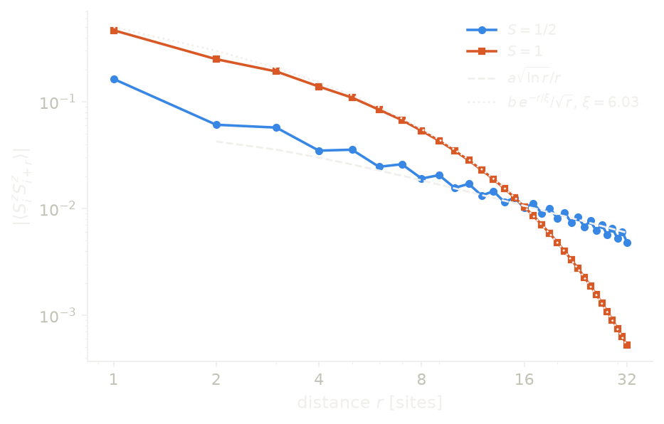
The figure shows \(|\langle S^z_iS^z_{i+r}\rangle|\) in two open Heisenberg chains with \(n=64\), measured from site \(i=16\). The spin-1/2 chain is gapless, and its correlations decay as a power law, \(\sqrt{\ln r}/r\) (dashed line). The small zigzag between even and odd \(r\) is an effect of the open ends. The spin-1 chain has the Haldane gap, and its correlations decay exponentially, as \(e^{-r/\xi}/\sqrt r\) with \(\xi=6.03\) (dotted line). A free fit of the DMRG data gives \(\xi=6.09\). In the spin-1 chain, the two end sites are spin 1/2. They bind the edge states of the open chain, so that the ground state is unique.
Code of this figure (docs/figures/ground-state_correlators/)
# <Sz_i Sz_{i+r}> in the open spin-1/2 and spin-1 Heisenberg chains, from the
# site i0 = n/2-16 outwards, so both sites stay 16 or more sites from the ends.
import numpy as np
from dmrgpy import spinchain

n = 64
rs = np.arange(1, 33)
i0 = n//2 - 16


def correlator(sites, maxm):
    sc = spinchain.Spin_Chain(sites)
    sc.set_hamiltonian(sum(sc.Sx[i]*sc.Sx[i+1] + sc.Sy[i]*sc.Sy[i+1]
                           + sc.Sz[i]*sc.Sz[i+1] for i in range(n-1)))
    sc.maxm, sc.nsweeps, sc.cutoff = maxm, 20, 1e-12
    sc.set_conserved_sector(Sz=0)
    return np.array([sc.vev(sc.Sz[i0]*sc.Sz[i0+r]).real for r in rs])


czz_half = correlator(["S=1/2"]*n, 120)
# A spin 1/2 at each end binds the free edge spins of the spin-1 chain into
# a singlet, so the ground state is unique and the bulk is unchanged.
czz_one = correlator(["S=1/2"] + ["S=1"]*(n-2) + ["S=1/2"], 100)

np.savez("data.npz", r=rs, czz_half=czz_half, czz_one=czz_one)
import numpy as np
import matplotlib.ticker as ticker
import style

d = np.load("data.npz")
r, czz_half, czz_one = d["r"], np.abs(d["czz_half"]), np.abs(d["czz_one"])
xi = 6.03  # Haldane correlation length
win = (r >= 8) & (r <= 32)  # fit window of the amplitudes a and b


def fit(c, f):
    """f times the amplitude fitted in log space on the window."""
    return np.exp(np.mean(np.log(c[win]) - np.log(f[win])))*f


ref_half = fit(czz_half, np.sqrt(np.log(r))/r)  # Luttinger liquid, log correction
ref_one = fit(czz_one, np.exp(-r/xi)/np.sqrt(r))  # Ornstein-Zernike, gapped
ok = r >= 2  # sqrt(ln r)/r vanishes at r=1
# xi fitted freely with the Ornstein-Zernike form, quoted in the guide
xi_free = -1/np.polyfit(r[win], np.log(czz_one[win]*np.sqrt(r[win])), 1)[0]


def draw(theme):
    c = style.colors(theme)
    fig, ax = style.figure(1)
    ax.plot(r, czz_half, "o-", color=c["series"][0], ms=4, label=r"$S=1/2$")
    ax.plot(r, czz_one, "s-", color=c["series"][1], ms=4, label=r"$S=1$")
    ax.plot(r[ok], ref_half[ok], **style.reference(theme),
            label=r"$a\sqrt{\ln r}/r$")
    ax.plot(r, ref_one, color=c["ink"], ls=":", lw=style.LW_REF,
            label=r"$b\,e^{-r/\xi}/\sqrt{r}$, $\xi=%.2f$" % xi)
    ax.set_xscale("log")
    ax.set_yscale("log")
    ax.set_xticks([1, 2, 4, 8, 16, 32])
    ax.xaxis.set_major_formatter(ticker.FormatStrFormatter("%g"))
    ax.xaxis.set_minor_formatter(ticker.NullFormatter())
    ax.set_xlabel(r"distance $r$ [sites]")
    ax.set_ylabel(r"$|\langle S^z_iS^z_{i+r}\rangle|$")
    ax.legend()
    return fig


style.main(draw, "ground-state_correlators")
Energy fluctuation
The energy variance tells us how close the state is to an eigenstate of \(H\):
de = sc.gs_energy_fluctuation()
For an exact eigenstate \(\delta E=0\). In DMRG, \(\delta E\) comes from the
truncation of the bond dimension, so it is a direct check of maxm. It is
a stricter check than the energy itself: roughly, the energy error is of
order \(\delta E^2\), while the error of other observables is of order
\(\delta E\). The figure in
Ground-state energy shows this on a Heisenberg
chain.
Fixed particle number or fixed magnetization
Without any constraint, DMRG returns the global ground state, at whatever particle number or total \(S^z\) it has. When \(H\) conserves a charge \(Q\), we can instead ask for the ground state of one sector,
Here fc is a Fermionic_Chain and hc a Spinful_Fermionic_Chain_Native.
fc.set_conserved_sector(Nf=6)          # exactly 6 fermions
sc.set_conserved_sector(Sz=0)          # total Sz = 0
hc.set_conserved_sector(Nf=8, Sz=0)    # Hubbard chain: both
fc.set_conserved_sector()              # back to the full Hilbert space
Sz is given in units of \(1/2\), so Sz=2 means \(S^z_\mathrm{tot}=1\).
The available charges are Nf for fermions, Sz for spins, both for the
native Hubbard chain, and Nb for bosons. Parafermion chains have none.
With sectors we compute the addition spectrum \(E_0(N)\), the charge gap
\(E_0(N+1)+E_0(N-1)-2E_0(N)\), and the magnetization curve, each point being
a true ground state of its own sector. The same calls work with
mode="ED". On large chains a sector is also faster, by about 4 times at
\(n=60\).
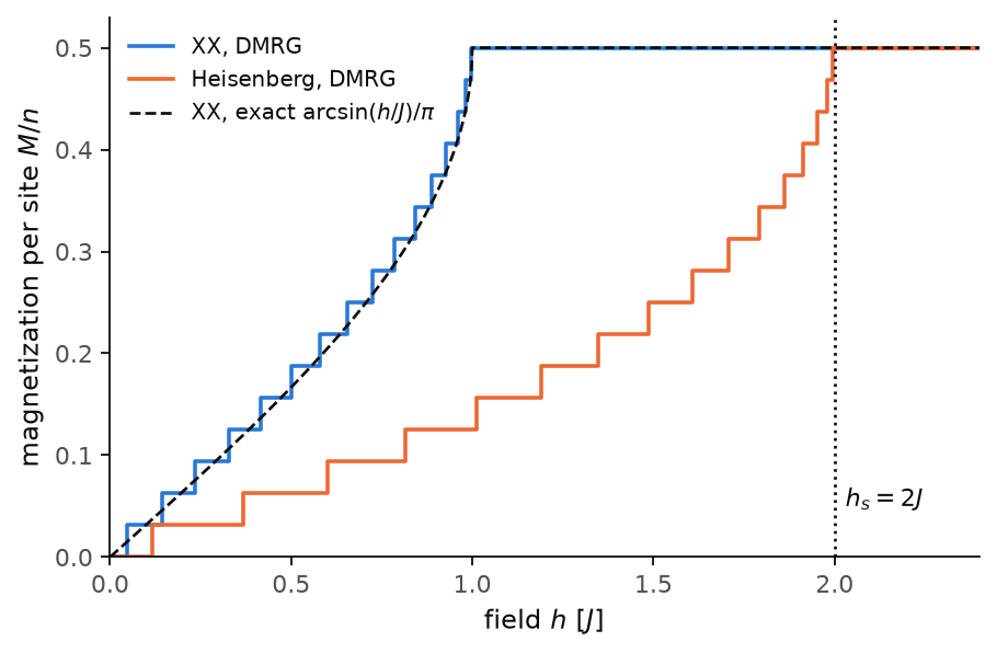
The figure shows the magnetization curve of two open chains with \(n=32\). In a field \(h\), the ground state is in the sector \(M=S^z_\mathrm{tot}\) that minimizes \(E_0(M)-hM\). So the magnetization jumps from \(M\) to \(M+1\) at \(h_M=E_0(M+1)-E_0(M)\), and one solve per sector gives the whole curve. For the XX chain (\(S^xS^x+S^yS^y\)) the steps follow the free-fermion curve \(\arcsin(h/J)/\pi\) (dashed line), and every \(E_0(M)\) agrees with free fermions on the same chain within \(3\times10^{-10}\). The Heisenberg chain saturates close to \(h_s=2J\); on this open chain the last step is at \(J(1+\cos(\pi/n))=1.995\,J\).
Code of this figure (docs/figures/ground-state_sectors/)
# Ground-state energies E0(M) of the open spin-1/2 XX and Heisenberg chains in
# every sector of total Sz = M; in a field h the magnetization steps from M to
# M+1 at h_M = E0(M+1) - E0(M).
import numpy as np
from dmrgpy import spinchain

n = 32
Ms = np.arange(0, n//2 + 1)


def sector_energy(heisenberg, M):
    sc = spinchain.Spin_Chain(["S=1/2"]*n)
    h = sum(sc.Sx[i]*sc.Sx[i+1] + sc.Sy[i]*sc.Sy[i+1] for i in range(n-1))
    if heisenberg:
        h = h + sum(sc.Sz[i]*sc.Sz[i+1] for i in range(n-1))
    sc.set_hamiltonian(h)
    sc.maxm, sc.nsweeps, sc.cutoff = 60, 12, 1e-12
    sc.set_conserved_sector(Sz=2*int(M))  # Sz in units of 1/2
    return sc.gs_energy()


e_xx = np.array([sector_energy(False, M) for M in Ms])
e_heis = np.array([sector_energy(True, M) for M in Ms])

# XX chain as free fermions with hopping J/2: E0(M) is the sum of the lowest
# n/2+M levels J cos(pi k/(n+1))
eps = np.sort(np.cos(np.pi*np.arange(1, n+1)/(n+1)))
e_xx_ff = np.array([np.sum(eps[:n//2 + M]) for M in Ms])

np.savez("data.npz", n=n, M=Ms, e_xx=e_xx, e_heis=e_heis, e_xx_ff=e_xx_ff)
import numpy as np
import style

d = np.load("data.npz")
n, M = d["n"], d["M"]
HMAX = 2.4


def staircase(e):
    """m(h) as a step curve: M for h between h_{M-1} and h_M."""
    x = np.concatenate([[0.0], np.diff(e), [HMAX]])  # h_M = E0(M+1) - E0(M)
    y = np.concatenate([M, [M[-1]]])/n
    return x, y


def draw(theme):
    c = style.colors(theme)
    fig, ax = style.figure(1)
    ax.step(*staircase(d["e_xx"]), where="post", color=c["series"][0],
            label="XX, DMRG")
    ax.step(*staircase(d["e_heis"]), where="post", color=c["series"][1],
            label="Heisenberg, DMRG")
    h = np.linspace(0, 1, 400)
    ax.plot(np.append(h, HMAX), np.append(np.arcsin(h)/np.pi, 0.5),
            **style.reference(theme), label=r"XX, exact $\arcsin(h/J)/\pi$")
    ax.axvline(2.0, color=c["ink"], ls=":", lw=style.LW_REF)
    ax.text(2.03, 0.05, r"$h_s=2J$", color=c["ink"])
    ax.set_xlim(0, HMAX)
    ax.set_ylim(0, 0.53)
    ax.set_xlabel(r"field $h$ [$J$]")
    ax.set_ylabel(r"magnetization per site $M/n$")
    ax.legend(loc="upper left")
    return fig


style.main(draw, "ground-state_sectors")
Inside a sector, every operator must conserve the charge. An operator that changes it, for example \(c_i\) at fixed \(N_f\) or \(S^x_i\) at fixed \(S^z\), raises an error. To apply such an operator to the sector ground state, first convert the state to an ordinary MPS:
fc.set_conserved_sector(Nf=6)
fc.gs_energy()
fc.promote_to_dense()                    # same state, no sector
wf = fc.applyoperator(fc.C[3], fc.wf0)   # c_3 |GS_N>, now with 5 fermions
Two ground states with \(N\) and \(N-1\) fermions, both converted this way, can
be compared directly. This gives for example the photoemission weight
\(Z_i=|\langle\mathrm{GS}_{N-1}|c_i|\mathrm{GS}_N\rangle|^2\)
(see examples/groundstate/sector_promotion_to_dense).
Backends
Sectors work on itensor_version=3, "python", "julia_live" and
mode="ED". They are not available on itensor_version=2, with METTS
and for infinite chains; these raise an error.