Excited states and gaps
On this page we compute the low-energy spectrum: excited states, gaps,
the degeneracy of the ground state, non-Hermitian and generalized
eigenproblems, and effective Hamiltonians of a low-energy manifold. Here sc is the Heisenberg chain of Ground state.
Low-lying spectrum
The lowest eigenvalues \(E_0\le E_1\le\dots\) of \(H\) and the gap \(\Delta=E_1-E_0\) are
es = sc.get_excited(n=4)                 # [E0, E1, E2, E3]
gap = sc.get_gap()                       # E1 - E0
es, ws = sc.get_excited_states(n=4)      # energies and states
The list has one entry per eigenstate, so a degenerate level appears once
for each state of the multiplet. If the ground state is degenerate,
get_gap() is zero, and we must ask for enough states to reach the first
excited level. When DMRG splits a multiplet slightly, identify the states
by a quantum number (for example \(\langle\mathbf S^2\rangle\)) and not by
their position in the list.
DMRG finds each excited state as the ground state of \(H\) plus a penalty
on the states already found. This search can converge to a wrong state.
When the energy variance of a state is much larger than that of the ground
state, a warning is printed, and the state should be checked with more
sweeps, a larger maxm or mode="ED" on a smaller chain. The keywords are:
n: the number of states.scale: the weight of the penalty, in units of the bandwidth of \(H\) (default 10).purify=True(default,get_excited_states): diagonalizes \(H\) again in the space of the states found, which separates nearly degenerate states.
For example, an open spin-1 Heisenberg chain has four low states from the two spin-1/2 edge modes (a singlet and a triplet), and the Haldane gap is the gap to the next state:
es = s1.get_excited(n=6)    # s1: an open spin-1 Heisenberg chain
haldane_gap = es[4] - es[0]
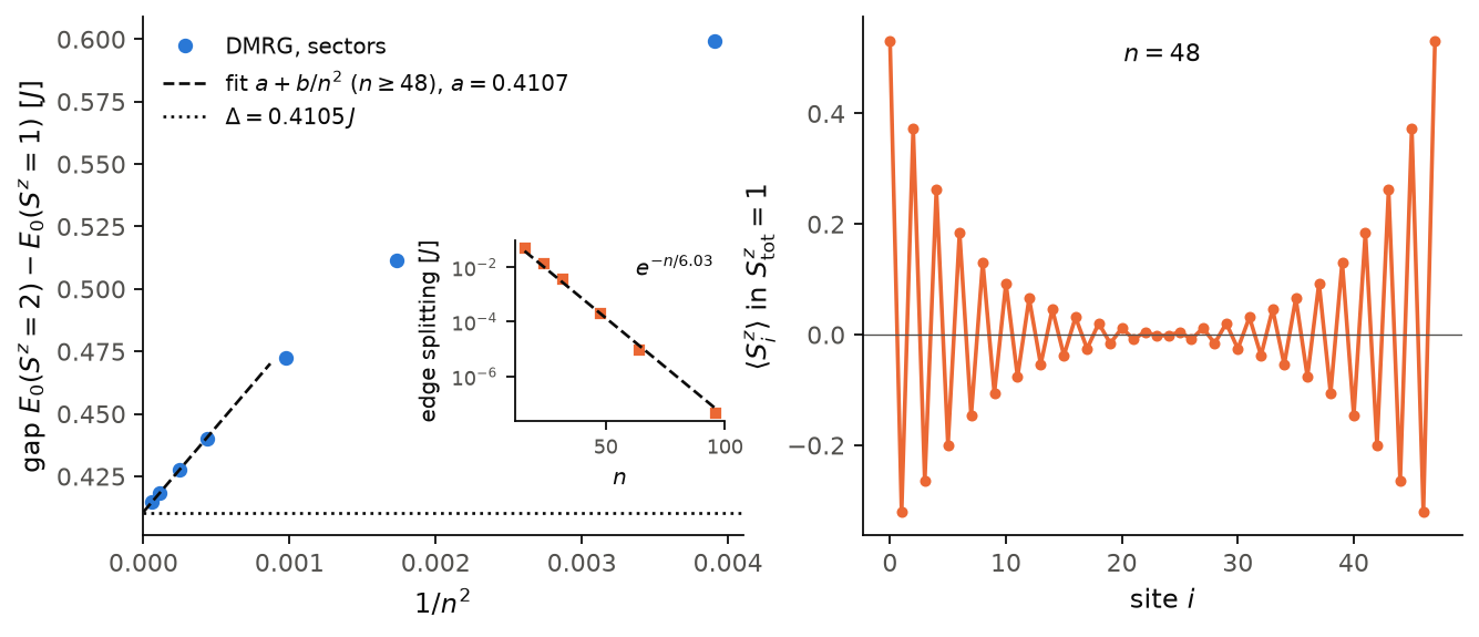
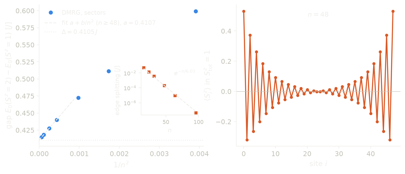
The figure shows the same physics on long open spin-1 chains. Here the
energies come from the ground states of three
sectors,
\(S^z_\mathrm{tot}=0\), 1 and 2, which is faster and safer than
get_excited at these lengths. The edge splitting is \(E_0(1)-E_0(0)\) and
the bulk gap is \(E_0(2)-E_0(1)\), one magnon on top of the edge triplet.
On the left, the gap goes as \(1/n^2\), and the fit \(a+b/n^2\) on
\(n=48\) to 128 gives \(0.4107\,J\), against the known \(\Delta=0.4105\,J\).
The inset shows that the edge splitting falls as \(e^{-n/\xi}\) with
\(\xi\approx6\), to below \(10^{-7}\) at \(n=96\), so the four edge states
become degenerate. On the right is \(\langle S^z_i\rangle\) in the
\(S^z_\mathrm{tot}=1\) ground state at \(n=48\). Each end carries a spin 1/2
(each half sums to exactly \(1/2\)), spread over about 6 sites, and the
bulk is not magnetized.
Code of this figure (docs/figures/excited-states_haldane/)
# Edge states and bulk gap of the open spin-1 Heisenberg chain, from the
# ground states of the sectors Sz_tot = 0, 1 and 2 (the two spin-1/2 edge
# states form a singlet and a triplet, the gap is a magnon on the triplet).
import numpy as np
from dmrgpy import spinchain

ns = [16, 24, 32, 48, 64, 96, 128]
n_profile = 48  # length of the <Sz_i> profile


def sector(n, sz):
    sc = spinchain.Spin_Chain(["S=1"]*n)
    sc.set_hamiltonian(sum(sc.Sx[i]*sc.Sx[i+1] + sc.Sy[i]*sc.Sy[i+1]
                           + sc.Sz[i]*sc.Sz[i+1] for i in range(n-1)))
    sc.maxm, sc.nsweeps, sc.cutoff = 150, 30, 1e-12
    sc.set_conserved_sector(Sz=2*sz)  # Sz is given in units of 1/2
    return sc, sc.gs_energy()


e0, e1, e2 = [], [], []
for n in ns:
    e0.append(sector(n, 0)[1])
    sc1, e = sector(n, 1)
    e1.append(e)
    e2.append(sector(n, 2)[1])
    if n == n_profile:
        profile = [sc1.vev(sc1.Sz[i]).real for i in range(n)]

np.savez("data.npz", ns=ns, e0=e0, e1=e1, e2=e2, profile=profile)
import numpy as np
import style

d = np.load("data.npz")
ns, prof = d["ns"], d["profile"]
x = 1.0/ns**2
gap = d["e2"] - d["e1"]          # bulk gap, one magnon on the edge triplet
split = np.abs(d["e1"] - d["e0"])  # edge splitting
gap_ref, xi = 0.41048, 6.03        # infinite chain (White and Huse)
# fit gap = a + b/n^2, weighted by n^2, on n >= 48 (next correction is 1/n^3)
nmin = 48
fit = ns >= nmin
gap_inf, slope = np.polynomial.polynomial.polyfit(x[fit], gap[fit], 1,
                                                  w=ns[fit]**2)
# prefactor of exp(-n/xi) on the splittings above 1e-9 (below, the
# sector energies are not accurate enough)
ok = split > 1e-9
pref = np.exp(np.mean(np.log(split[ok]) + ns[ok]/xi))


def draw(theme):
    c = style.colors(theme)
    fig, (a1, a2) = style.figure(2)
    xx = np.linspace(0, 2.0/nmin**2, 50)
    a1.plot(x, gap, "o", color=c["series"][0], label="DMRG, sectors")
    a1.plot(xx, gap_inf + slope*xx, **style.reference(theme),
            label=r"fit $a+b/n^2$ ($n\geq%d$), $a=%.4f$" % (nmin, gap_inf))
    a1.axhline(gap_ref, color=c["ink"], ls=":", lw=style.LW_REF,
               label=r"$\Delta=0.4105\,J$")
    a1.set_xlabel(r"$1/n^2$")
    a1.set_ylabel(r"gap $E_0(S^z{=}2)-E_0(S^z{=}1)$ [$J$]")
    a1.set_xlim(left=0)
    a1.legend(loc="upper left")
    ins = a1.inset_axes([0.62, 0.22, 0.35, 0.35])
    ins.plot(ns[ok], split[ok], "s", color=c["series"][1], ms=4)
    nn = np.linspace(ns.min(), ns[ok].max(), 50)
    ins.plot(nn, pref*np.exp(-nn/xi), **style.reference(theme))
    ins.text(0.95, 0.92, r"$e^{-n/6.03}$", transform=ins.transAxes,
             ha="right", va="top", fontsize=9)
    ins.set_yscale("log")
    ins.set_xlabel(r"$n$", fontsize=9)
    ins.set_ylabel(r"edge splitting [$J$]", fontsize=9)
    ins.tick_params(labelsize=8)
    a2.plot(np.arange(len(prof)), prof, "o-", color=c["series"][1], ms=3.5)
    a2.axhline(0, color=c["ink2"], lw=0.6)
    a2.set_xlabel(r"site $i$")
    a2.set_ylabel(r"$\langle S^z_i\rangle$ in $S^z_{\rm tot}=1$")
    a2.text(0.5, 0.95, r"$n=%d$" % len(prof), transform=a2.transAxes,
            ha="center", va="top")
    return fig


style.main(draw, "excited-states_haldane")
Ground-state degeneracy
A degenerate ground state signals a broken symmetry or a topological phase. Examples are the two ordered states of an Ising chain and the four edge states of an open Haldane chain, whose splitting is shown in Low-lying spectrum. We count the levels close to \(E_0\),
adding excited states \(E_i\) until the count stops growing:
g = sc.get_gs_degeneracy()             # close to an integer
g = sc.get_gs_degeneracy(delta=1e-4)   # a stricter window
A level counts when \(|E_i-E_0|\) is smaller than about \(\sqrt{\delta}\),
which is 0.1 at the default delta=1e-2. A result that is not close to
an integer means that a level sits at the edge of the window. On a finite
chain a degeneracy is often split by an amount that decays with the
length, so choose delta relative to that splitting. mode="ED" uses
exact diagonalization.
The states of the manifold are sc.get_gs_manifold(n=2, tol=1e-3), the
eigenstates within tol of \(E_0\) (more states are searched when all n
turn out degenerate), and sc.vev(A, wf=w) measures an operator in any
of them. Here sc is an Ising chain
\(H=-\sum_iS^z_iS^z_{i+1}-0.2\sum_iS^x_i\) in its ordered phase:
wfs = sc.get_gs_manifold(n=2, tol=1e-3)         # two states
M = sum(sc.Sz)
print([sc.vev(M, wf=w).real for w in wfs])      # 0 and 0
print(sc.aMb(wfs[0], M, wfs[1]).real)           # modulus 4.82 on 10 sites
up = sc.summps(wfs[0], wfs[1]).normalize()      # the ordered states
dn = sc.summps(wfs[0], -1*wfs[1]).normalize()
print(sc.vev(M, wf=up).real, sc.vev(M, wf=dn).real)   # 4.82 and -4.82, in some order
The eigenstates are the symmetric and antisymmetric combinations of the
two ordered states, so the magnetization vanishes in each of them and
appears in the off-diagonal element. The ordered states are their sum
and difference. The dynamical correlator
with mode="ED" averages over such a manifold by itself.
Gap to another particle number
For a conserved charge \(A\), for
example the particle number \(N=\sum_in_i\), get_charge_gap(d=...) gives
the energy to change \(\langle A\rangle\) by \(d\) from its ground-state value
\(A_0\). It solves
increasing \(\lambda\) until the constraint holds, and returns \(\Delta(d)=E_0(A_0+d)-E_0(A_0)\).
gap2 = fc.get_charge_gap(d=2) # fc: a fermionic chain; add two particles
d=2 is the cost of adding a pair, and d=-2 of removing one.
Fermionic_Chain, Spinful_Fermionic_Chain and the native spinful chain
have this method. The conserved sectors give the same energies
directly, \(E_0(N)\) for each \(N\).
Non-Hermitian Hamiltonians
When \(H\neq H^\dagger\) (gain and loss, complex or non-reciprocal hopping), the ground state is the eigenvalue with the smallest real part. Eigenstates come in left and right pairs,
gs_energy() detects a non-Hermitian \(H\). With mode="DMRG" it evolves a
random state in imaginary time with \(H\) itself,
\(|\psi(\tau)\rangle\propto e^{-\tau H}|\psi(0)\rangle\), normalized at every
step. The levels of smallest real part grow fastest, so the state ends in
their span. Several levels often share that real part, for example a
complex-conjugate pair in a PT-symmetric chain. Then the state keeps
rotating between them, so the energies are read from a small
diagonalization of \(H\) in the span of the last states of the evolution.
The left state comes from the same evolution with \(H^\dagger\). Here fc
is a fermionic chain with a non-Hermitian Hamiltonian, for example a
staggered imaginary potential \(i\gamma(-1)^in_i\):
e = fc.gs_energy()              # E; stores the right state as the ground state
es, res = fc.get_nh_levels()    # the levels of smallest real part, with residuals
e, psil, psir = fc.nhdmrg()     # non-Hermitian DMRG: E, left and right states
get_nh_levels() returns every level it finds, sorted by real part, with
its relative residual. When the spectrum is degenerate in the real part,
the first entries are all the levels that share it, which a single
eigenpair cannot show. vectors=True also returns their right states. A
level in a symmetry sector the random start has no weight in does not
appear. nhdmrg() is non-Hermitian DMRG (NH-DMRG), which returns one
left and right pair.
The energy is not a variational bound, so the result is checked with the residuals \(\lVert H|\psi_R\rangle-E|\psi_R\rangle\rVert\) and \(\lVert H^\dagger|\psi_L\rangle-E^*|\psi_L\rangle\rVert\). The keywords are:
tol: the largest relative residual accepted (default1e-4).ntries: how many times NH-DMRG restarts from a random state when the residual is too large (default 5).fc.nh_gs_method(default"imaginary_time"):"nhdmrg"makesgs_energy()use NH-DMRG. NH-DMRG is faster where it converges, and the imaginary-time route also runs it when its own result fails the residual check, keeping the better of the two.fc.maxm: the state has to hold all the levels that share the real part at once, so a multiplet of many tied levels needs a larger bond dimension than one level does. Raise it when the check fails.
Backends
The imaginary-time route and get_nh_levels() run on
itensor_version=3 and "python", without a conserved sector. On the
other backends gs_energy() uses NH-DMRG, which works on
itensor_version=2, 3, "python" and "julia_live".
See examples/non_hermitian/nh_levels_imaginary_time, where the four
levels of smallest real part of a PT-symmetric XX chain come out together.
Excited states of a non-Hermitian \(H\) come from get_excited_states(n) and
get_excited(n), which use an Arnoldi method on matrix product states. It
is less accurate than NH-DMRG, so check it against mode="ED" on a small
chain (examples/non_hermitian/nhdmrg_VS_ED_VS_arnoldi).
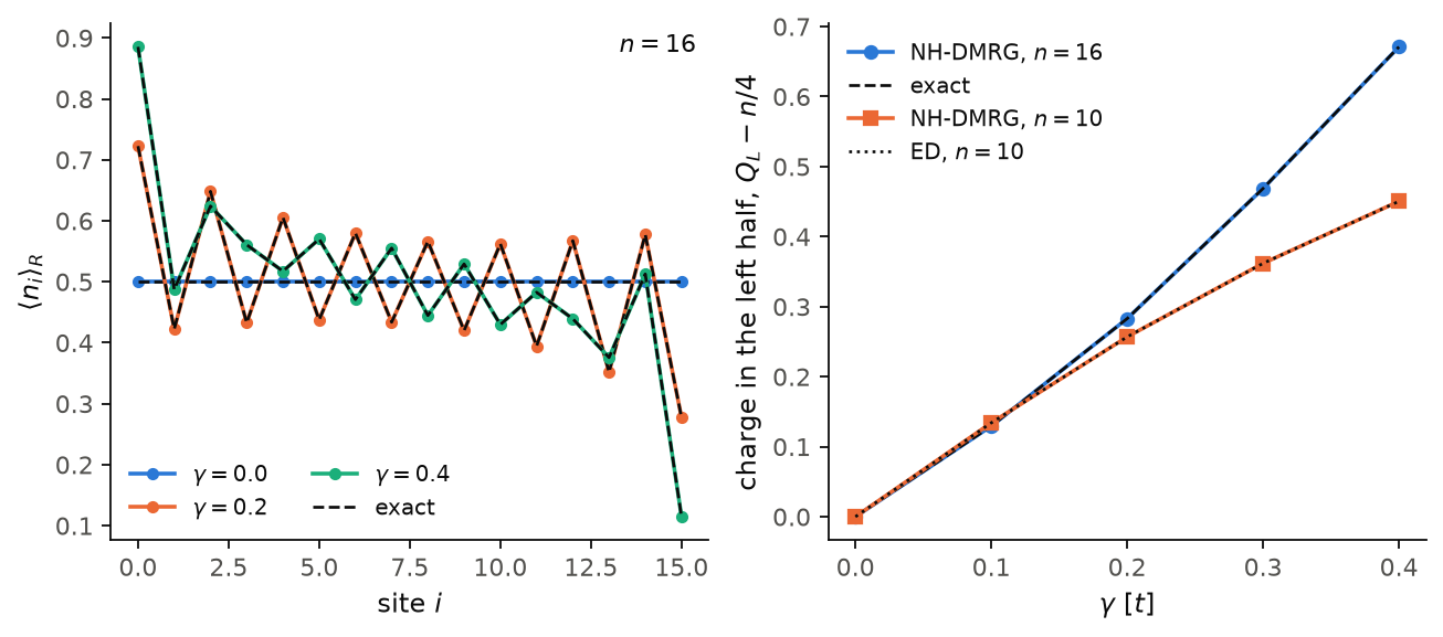
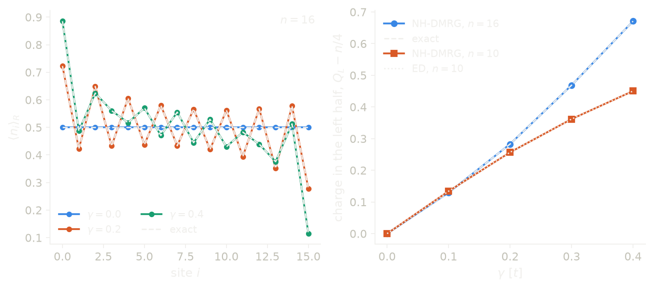
The figure shows the many-body skin effect of an interacting
Hatano-Nelson chain at half filling, with hopping \(t\pm\gamma\) and a
nearest-neighbor repulsion \(V=t\). On the left is the density of the right
ground state, \(\langle\psi_R|n_i|\psi_R\rangle/\langle\psi_R|\psi_R\rangle\),
from nhdmrg() on 16 sites. It is flat at \(\gamma=0\), and charge moves to
the left end as \(\gamma\) grows. On the right is the charge moved into the
left half. The dashed curves are exact, since with open ends \(H\) is a
similarity transform of a Hermitian chain, and ED on 10 sites agrees with
NH-DMRG to \(10^{-14}\). The problem becomes ill conditioned fast with \(n\)
and \(\gamma\); nhdmrg warns when it does not converge, and again each
time the unconverged state is used.
Code of this figure (docs/figures/excited-states_nonhermitian/)
# Many-body skin effect of the interacting Hatano-Nelson chain, from NH-DMRG.
# With open ends H = S H0 S^-1, with H0 the chain with symmetric hopping
# t' = sqrt((t+g)(t-g)) and S = prod_j r^(j n_j), r = t'/(t+g): this is the
# exact reference at n sites, and ED is the reference at n_ed sites.
import numpy as np
from dmrgpy import fermionchain

t, V = 1.0, 1.0
gammas = [0.0, 0.1, 0.2, 0.3, 0.4]
n, n_ed = 16, 10


def chain(n, tl, tr):  # tl on c^dag_i c_i+1, tr on c^dag_i+1 c_i
    fc = fermionchain.Fermionic_Chain(n)
    fc.set_hamiltonian(sum(tl*fc.Cdag[i]*fc.C[i+1] + tr*fc.Cdag[i+1]*fc.C[i]
                           + V*(fc.N[i]-0.5)*(fc.N[i+1]-0.5)
                           for i in range(n-1)))
    fc.maxm, fc.nsweeps, fc.cutoff = 80, 20, 1e-12
    return fc


def density(fc, wf, **kw):  # right-vector density <n_i>_R
    norm = fc.aMb(wf, fc.Id, wf, **kw).real
    return [fc.aMb(wf, fc.N[i], wf, **kw).real/norm for i in range(len(fc.N))]


def nh_solve(n, g):
    fc = chain(n, t+g, t-g)
    e, psil, psir = fc.nhdmrg(tol=1e-5, ntries=3)
    res = fc.applyoperator(fc.hamiltonian, psir) - e*psir
    resid = np.sqrt(abs(res.overlap(res))/abs(psir.overlap(psir)))/abs(e)
    return e.real, density(fc, psir), resid


def reference(n, g):
    tp = np.sqrt((t+g)*(t-g))
    fh = chain(n, tp, tp)
    e0, w = fh.gs_energy(), fh.get_gs()
    for j in range(n):  # S, centred to keep the numbers of order one
        w = fh.applyoperator(fh.Id + ((tp/(t+g))**(j-(n-1)/2.)-1)*fh.N[j], w)
    return e0, density(fh, w)


dens, dens_ref, dens_small, dens_ed, converged = [], [], [], [], []
for g in gammas:
    dens_small.append(nh_solve(n_ed, g)[1])
    fe = chain(n_ed, t+g, t-g)
    _, ws = fe.get_excited_states(mode="ED", n=1)
    dens_ed.append(density(fe, ws[0], mode="ED"))
    e, d, resid = nh_solve(n, g)
    e0, dref = reference(n, g)
    dens.append(d)
    dens_ref.append(dref)
    converged.append(abs(e - e0) < 1e-6 and resid < 1e-4)  # else not plotted

np.savez("data.npz", gamma=gammas, n=n, n_ed=n_ed, dens=dens,
         dens_ref=dens_ref, dens_small=dens_small, dens_ed=dens_ed,
         converged=converged)
import numpy as np
import style

d = np.load("data.npz")
gam, n, n_ed = d["gamma"], int(d["n"]), int(d["n_ed"])
conv = d["converged"].astype(bool)  # a failed NH-DMRG solve is left out
SHOW = [0.0, 0.2, 0.4]              # the g of the left panel


def left_charge(dens):  # charge moved into the left half
    m = dens.shape[-1]
    return dens[..., :m//2].sum(axis=-1) - m/4


def draw(theme):
    c = style.colors(theme)
    fig, (a1, a2) = style.figure(2)
    shown = [k for k, g in enumerate(gam) if conv[k] and
             np.min(np.abs(g - np.array(SHOW))) < 1e-9]
    i = np.arange(n)
    for j, k in enumerate(shown):
        a1.plot(i, d["dens"][k], "o-", color=c["series"][j], ms=4,
                label=r"$\gamma=%.1f$" % gam[k])
        a1.plot(i, d["dens_ref"][k], **style.reference(theme),
                label="exact" if j == len(shown)-1 else None)
    a1.set_xlabel(r"site $i$")
    a1.set_ylabel(r"$\langle n_i\rangle_R$")
    a1.legend(loc="lower left", ncol=2)
    a1.text(0.98, 0.98, r"$n=%d$" % n, transform=a1.transAxes,
            ha="right", va="top")

    a2.plot(gam[conv], left_charge(d["dens"])[conv], "o-",
            color=c["series"][0], label=r"NH-DMRG, $n=%d$" % n)
    a2.plot(gam, left_charge(d["dens_ref"]), **style.reference(theme),
            label="exact")
    a2.plot(gam, left_charge(d["dens_small"]), "s-", color=c["series"][1],
            label=r"NH-DMRG, $n=%d$" % n_ed)
    a2.plot(gam, left_charge(d["dens_ed"]), color=c["ink"], ls=":",
            lw=style.LW_REF, label=r"ED, $n=%d$" % n_ed)
    a2.set_xlabel(r"$\gamma$ [$t$]")
    a2.set_ylabel(r"charge in the left half, $Q_L-n/4$")
    a2.legend(loc="upper left")
    return fig


style.main(draw, "excited-states_nonhermitian")
Spectrum from time evolution
We will now see a second way to get several low eigenvalues at once, for a Hermitian or a non-Hermitian \(H\). We evolve two random states in imaginary time, \(|\rho_m\rangle=e^{Gzm}|\rho_0\rangle\) with \(G=-H\), and keep every snapshot. One state evolves along \(z=\delta t\), the other along the complex contour \(z=\delta t\,e^{-i\alpha}\), which slows down the decay of modes with \(\mathrm{Im}\,\lambda>0\). Then we diagonalize \(G\) in the space spanned by the snapshots. The eigenvalues \(\lambda\) with the largest real part come first, so for \(G=-H\) the energies are \(E=-\lambda\), lowest first. This is the method of arXiv:2509.07709, where \(G\) is a Lindbladian.
sc = spinchain.Spin_Chain(["S=1/2" for i in range(n)], itensor_version="python")
sc.set_hamiltonian(h)
ev, res, obs = sc.get_krylov_spectrum()  # eigenvalues of G = -H
es = -ev                                 # energies, lowest first
zz = obs(sc.Sz[0]*sc.Sz[1], 0)           # <Sz0 Sz1> in the lowest state
res[k] says how much \(\lambda_k\) moves when the last snapshot of each
state is left out. A converged eigenvalue does not move, so a small
res[k] marks the converged part of the list. It is not an error bar: on
small chains the true error was 3 to 40 times larger. On the 20-site
chain the lowest energy agrees with gs_energy() to \(10^{-5}\). For a Hermitian \(H\) each energy is an upper bound
on the exact one at the same position. Two random starts give at most two
copies of a degenerate level, so a triplet appears twice. The keywords are:
G: the generator, aMultiOperator(default \(-H\)).nk: the number of snapshots per state (default 20).dt: the time step (default 0.5). A smalldtgives snapshots that are almost parallel, and the spectrum becomes worse.alpha: the contour angle (default: estimated from a short run).gram_tol: relative threshold below which directions of the snapshot space are dropped (default1e-12).exact_residuals=True:res[k]becomes the residual \(\lVert G|r_k\rangle-\lambda_k|r_k\rangle\rVert\) of the normalized eigenvector. It is a real error measure, but it costs much more on a large chain.mode="ED": every eigenvalue of the dense \(G\), in the same order, as a reference.
Backends
get_krylov_spectrum runs on itensor_version="python", 3 and
"julia_live", and not yet in a conserved sector. On "julia_live"
it takes random starts only. The random starts differ between the
backends, so the unconverged levels differ too.
Generalized eigenvalue problem
For a Hermitian positive definite operator \(A\),
A = fc.Id + 0.5*sum(fc.N)           # for example
lam = fc.gs_energy_generalized(A)   # smallest lambda
DMRG solves this directly, with no inverse of \(A\). A non-Hermitian \(H\) is
also accepted, and then \(\lambda\) is the complex eigenvalue with the
smallest real part. Not available on itensor_version=2, it raises an
error. It also raises if \(A\) is not Hermitian, or if \(\langle\psi|A|\psi\rangle\)
is not positive during the solve.
After this call the chain stores the generalized eigenstate as its ground
state, and fc.e0 is its energy
\(\langle\psi|H|\psi\rangle/\langle\psi|\psi\rangle\) (with left and right
states for a non-Hermitian \(H\)), while \(\lambda\) is in
fc.lam_generalized. Every later calculation (excited states,
correlators) uses this state. So call it last, or call fc.restart() and
fc.gs_energy() to get back the true ground state.
Effective low-energy Hamiltonians
An effective Hamiltonian acts in a small model space and has the same low-energy spectrum as \(H\). For a Hubbard chain at strong coupling the model space is the states with one electron per site, and the effective model is a spin model. We take the \(n\) lowest eigenstates \(|\psi_k\rangle\), project them on the model space with its projector \(Q\), and orthonormalize them (Löwdin), which gives \(|\tilde k\rangle\). The effective Hamiltonian is
and the couplings \(J_a\) of the operators \(O_a\) are fitted by least squares, with the \(O_a\) represented on the \(|\tilde k\rangle\). This is the des Cloizeaux effective Hamiltonian. It has the eigenvalues \(E_k\), so on a Hubbard dimer the fitted exchange is the singlet-triplet splitting \(E_T-E_S\), which tends to \(4t^2/U\) at strong coupling:
# fc: a Spinful_Fermionic_Chain(2) Hubbard dimer, with 20*(N-2)^2 added
# to H to keep the four lowest states at half filling
from dmrgpy import effectivehamiltonian
Q = effectivehamiltonian.single_occupancy_projector(fc)
J = fc.get_heff(operators=[fc.Sx[0]*fc.Sx[1], fc.Sy[0]*fc.Sy[1],
                           fc.Sz[0]*fc.Sz[1]], n=4, projector=Q)

coef = effectivehamiltonian.get_effective_hamiltonian_couplings(fc, n=4,
                                                               projector=Q)
latex = effectivehamiltonian.get_effective_hamiltonian(fc, n=4, projector=Q)
get_heff fits the operators given and returns one \(J\) per operator.
get_effective_hamiltonian_couplings
fits all products \(S^\alpha_iS^\beta_j\) of the chain spin operators and
returns a dictionary, and get_effective_hamiltonian returns the same fit
as a LaTeX string. The keywords are:
n: the number of states. It must not cut a degenerate multiplet, and it must not be larger than the dimension of the model space. Otherwise it raises an error.projector: the projector on the model space, as an operator or a list of commuting operators.single_occupancy_projector(fc)gives the states with one electron per site. Without it, the model space is the span of the \(n\) eigenstates themselves. This is right for a spin chain, but for a Hubbard chain the spin operators then miss the doubly occupied weight, and \(J\) is too large at small \(U\).operators: the operators of the fit. They must be linearly independent in the model space, otherwise the couplings are not unique and it raises an error.tol: couplings smaller than this are set to zero.method:"single"(default) fits \(QO_aQ\,QO_bQ\), and"full"fits \(Q\,O_aO_b\,Q\). They differ when the model space is not closed under \(O_a\).mode="ED": exact eigenstates, for small systems.
See examples/groundstate/effective_hamiltonian, which fits the twisted
exchange of a Hubbard dimer with a Peierls phase.
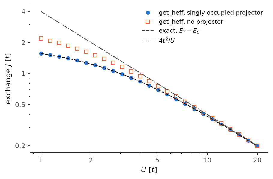
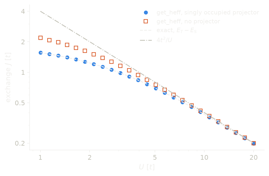
The figure shows the exchange \(J\) that get_heff fits on a Hubbard dimer
(n=4, mode="ED", with \(20(N-2)^2\) added to \(H\) to keep the four
states at half filling). The three couplings come out equal, as for an
isotropic exchange. With the projector, \(J\) is the splitting \(E_T-E_S\)
(dashed) at every \(U\), and it joins \(4t^2/U\) at large \(U\). Without the
projector, \(J\) is too large at small \(U\): the singlet has doubly occupied
weight, where \(\mathbf S_0\cdot\mathbf S_1=0\), and the fit gives
\((E_T-E_S)/(1/4+3w/4)\), with \(w\) the singly occupied weight. This is 40%
above the splitting at \(U=t\).
Code of this figure (docs/figures/excited-states_heff/)
# Exchange J of the half-filled Hubbard dimer, fitted by get_heff on the
# four lowest states, with and without projecting them on the singly
# occupied states.
import numpy as np
from dmrgpy import effectivehamiltonian, fermionchain

t = 1.0
lam = 20.0  # lam*(N-2)^2 keeps the four lowest states at half filling
Us = np.geomspace(1, 20, 25)

jfit, jfit_noproj = [], []
for U in Us:
    fc = fermionchain.Spinful_Fermionic_Chain(2)
    h = t*fc.Cdagup[0]*fc.Cup[1] + t*fc.Cdagdn[0]*fc.Cdn[1]
    h = h + h.get_dagger()
    h = h + sum(U*(fc.Nup[i]-0.5)*(fc.Ndn[i]-0.5) for i in range(2))
    ntot = fc.Ntot[0] + fc.Ntot[1]
    fc.set_hamiltonian(h + lam*(ntot-2)*(ntot-2))
    ops = [fc.Sx[0]*fc.Sx[1], fc.Sy[0]*fc.Sy[1], fc.Sz[0]*fc.Sz[1]]
    proj = effectivehamiltonian.single_occupancy_projector(fc)
    jfit.append(np.real(fc.get_heff(operators=ops, n=4, mode="ED",
                                    projector=proj)))
    jfit_noproj.append(np.real(fc.get_heff(operators=ops, n=4, mode="ED")))

np.savez("data.npz", t=t, U=Us, jfit=jfit, jfit_noproj=jfit_noproj)
import numpy as np
import matplotlib.ticker as ticker
import style

d = np.load("data.npz")
U, t = d["U"], d["t"]
j_exact = 0.5*(np.sqrt(U**2 + 16*t**2) - U)  # triplet-singlet splitting


def draw(theme):
    c = style.colors(theme)
    fig, ax = style.figure(1)
    ax.plot(U, d["jfit"][:, 2], "o", color=c["series"][0],
            label=r"get_heff, singly occupied projector")
    ax.plot(U, d["jfit_noproj"][:, 2], "s", mfc="none",
            color=c["series"][1], label=r"get_heff, no projector")
    ax.plot(U, j_exact, **style.reference(theme), label=r"exact, $E_T-E_S$")
    ax.plot(U, 4*t**2/U, color=c["ink2"], ls="-.", lw=style.LW_REF,
            label=r"$4t^2/U$")
    ax.set_xscale("log")
    ax.set_yscale("log")
    ax.set_xticks([1, 2, 5, 10, 20])
    ax.set_yticks([0.2, 0.5, 1, 2, 4])
    for axis in (ax.xaxis, ax.yaxis):
        axis.set_major_formatter(ticker.FormatStrFormatter("%g"))
        axis.set_minor_formatter(ticker.NullFormatter())
    ax.set_xlabel(r"$U$ [$t$]")
    ax.set_ylabel(r"exchange $J$ [$t$]")
    ax.legend()
    return fig


style.main(draw, "excited-states_heff")