Dynamical correlators
On this page we compute zero-temperature dynamical correlators: the dynamical spin structure factor, the single-particle spectral function and the local density of states, and the correlator of any pair of operators \((A,B)\).
The quantity
For a pair \((A,B)\), get_dynamical_correlator returns the
Lehmann spectral density
with \(M_n=\langle\mathrm{GS}|A|n\rangle\langle n|B|\mathrm{GS}\rangle\), \(\Delta_n=E_n-E_0\), and the resolvents \(G^{R/A}_{AB}(\omega)=\langle\mathrm{GS}|A\,(\omega+E_0\pm i\delta-H)^{-1}B|\mathrm{GS}\rangle\). The frequency \(\omega\) is measured from the ground-state energy \(E_0\), and \(\delta\) is the broadening. When every \(M_n\) is real, \(S_{AB}\) is real and equal to \(-\frac1\pi\mathrm{Im}\,G^R_{AB}(\omega)\). This is always the case for a Hermitian pair \(A=B^\dagger\), where \(S_{AB}\ge0\), and also for real operators on a real Hamiltonian. In general \(M_n\) is complex, so the returned array is complex. A converged calculation satisfies the sum rule
which is a simple check of a calculation. For EX and SECTOR (Choosing a correlator method) the
missing weight is the part of the spectrum outside the states kept. Here \(|\mathrm{GS}\rangle\) is the
ground state of the chain, or the state set with set_gs().
All the examples use the Heisenberg chain sc of Ground state.
import numpy as np
es = np.linspace(-1, 4, 300)                      # frequencies
(x, y) = sc.get_dynamical_correlator(name=(sc.Sz[0], sc.Sz[0]),
                                     es=es, delta=0.1)
print(np.sum(y.real)*(x[1]-x[0]))                 # sum rule: <Sz_0 Sz_0> = 0.25
The keywords that every method shares are:
name=(A, B): the operator pair, built from the chain operators. A string with two sites also works,name="ZZ", i=0, j=3, as do"XX","YY","+-","cdc"and"densitydensity".es: the frequency grid.delta: the broadening. A pole becomes a line of full width \(2\delta\).submode: the method, see Choosing a correlator method. The default is"KPM".mode="ED": exact diagonalization, for small chains and for checking. It accepts the submodes"KPM","ED","INV","EX","CVM","ROOTN"and"TD".
The default es and delta change from one method to another, so it is
best to always give them. A KPM line has the width \(2\delta\) at the
center of the many-body spectrum, and down to about 0.7 of it for low-energy
excitations of a long chain. It is not a Lorentzian: its peak is about 1.5
times higher than a Lorentzian of the same width and weight. So compare
peak heights only between calculations with the same method.
Dynamical spin structure factor
The dynamical spin structure factor is
The local one, \(i=j\), is what inelastic spin-flip spectroscopy with an STM measures on a single magnetic atom. Its Fourier transform
is what inelastic neutron scattering measures. We compute it from all the site pairs:
es = np.linspace(0, 4, 100)
qs = np.linspace(0, 2*np.pi, 41)
sqw = np.zeros((len(qs), len(es)))
for i in range(n):
    for j in range(n):
        (x, y) = sc.get_dynamical_correlator(name=(sc.Sz[i], sc.Sz[j]),
                                             es=es, delta=0.1)
        sqw += np.real(np.exp(1j*qs*(i-j))[:, None]*y[None, :])/n
For a Heisenberg chain the weight is largest at \(q=\pi\), the antiferromagnetic wave vector, and its lower edge follows the two-spinon dispersion \(\frac{\pi}{2}|\sin q|\) for long chains.
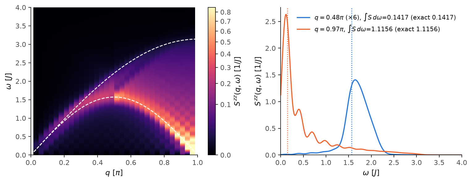
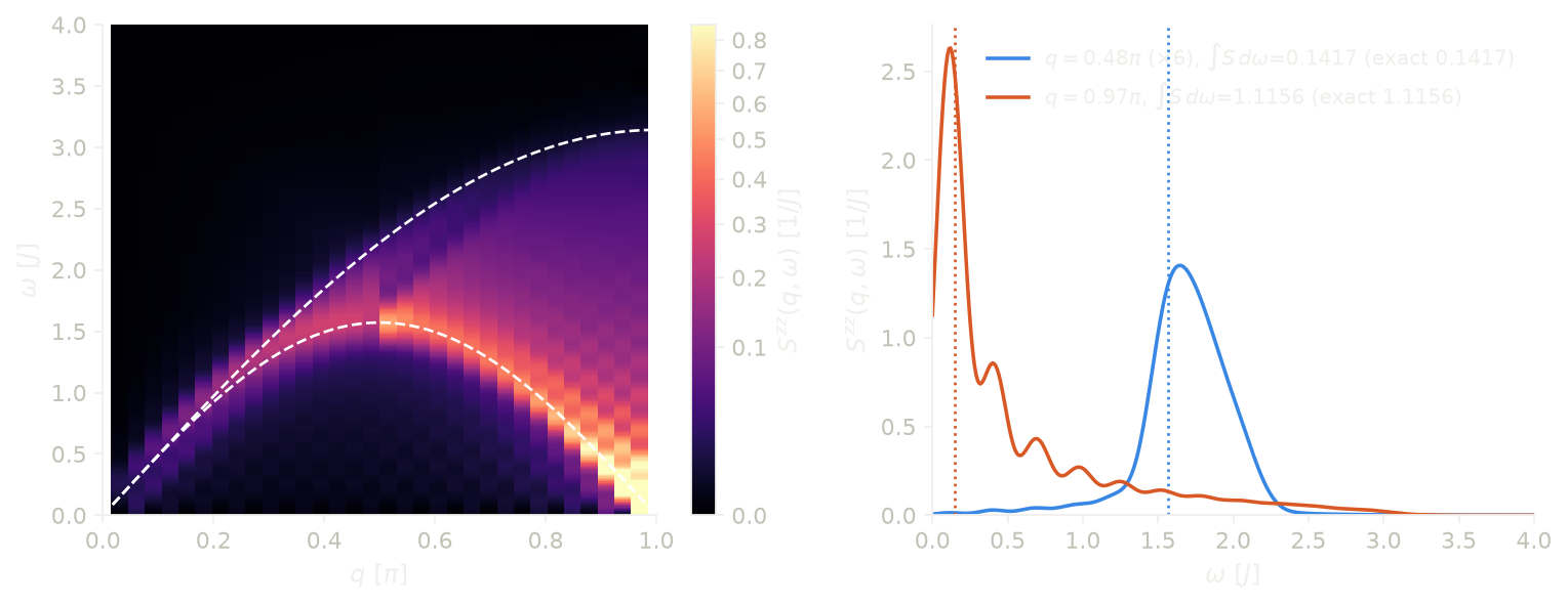
The figure shows \(S^{zz}(q,\omega)\) of an open Heisenberg chain with
\(n=32\), with KPM and \(\delta=0.15\). On an open chain the momentum states
are standing waves, so we use one operator per momentum,
\(S^z_q=\sqrt{2/(n+1)}\sum_i\sin(q(i+1))S^z_i\) with \(q=\pi k/(n+1)\), and one
KPM run per \(q\). The weight fills the two-spinon continuum between the
exact edges \(\frac{\pi}{2}J|\sin q|\) and \(\pi J|\sin(q/2)|\) (dashed). It is
largest just above the lower edge and near \(q=\pi\). The right panel shows
two cuts, with the lower edge as a dotted line. Their integrals match
\(\langle S^z_qS^z_q\rangle\) from vev. At every \(q\) this sum rule holds
to a few parts in \(10^5\).
Code of this figure (docs/figures/dynamical-correlators_sqw/)
# Dynamical spin structure factor S^zz(q,w) of the open spin-1/2 Heisenberg
# chain, one KPM run per momentum. On an open chain the momentum states are
# standing waves, S^z_q = sqrt(2/(n+1)) sum_i sin(q(i+1)) S^z_i, q = pi k/(n+1).
import numpy as np
from dmrgpy import spinchain, kpmdmrg

n = 32
delta = 0.15
es = np.linspace(0.0, 4.0, 400)
qs = np.pi*np.arange(1, n+1)/(n+1)

sc = spinchain.Spin_Chain(["S=1/2"]*n)
h = sum(sc.Sx[i]*sc.Sx[i+1] + sc.Sy[i]*sc.Sy[i+1] + sc.Sz[i]*sc.Sz[i+1]
        for i in range(n-1))
sc.set_hamiltonian(h)
sc.maxm, sc.nsweeps, sc.cutoff = 80, 14, 1e-12
sc.kpmmaxm = 40  # kpmmaxm=80 changes S(q,w) at q close to pi by less than 1%
sc.gs_energy()


def spectrum(x, mus, emin, emax, scale, npol, d):
    _, y = kpmdmrg.dynamical_correlator_from_moments(
        mus, emin, emax, scale, npol, x, kernel="jackson", delta=d,
        origin=sc.e0)
    return y.real


sqw, sumrule, sq = [], [], []
for q in qs:
    Sq = sum(np.sqrt(2/(n+1))*np.sin(q*(i+1))*sc.Sz[i] for i in range(n))
    m = sc.get_dynamical_correlator_moments(name=(Sq, Sq), delta=delta)
    sqw.append(spectrum(es, *m))
    # sum rule: the integral over the whole spectrum is <S^z_q S^z_q>
    ew = np.linspace(-1.0, m[2] - sc.e0 + 1.0, 20000)
    sumrule.append(np.trapezoid(spectrum(ew, *m), ew))
    sq.append(sc.vev(Sq*Sq).real)

np.savez("data.npz", qs=qs, es=es, sqw=sqw, sumrule=sumrule, sq=sq)
import numpy as np
from matplotlib.colors import PowerNorm
import style

d = np.load("data.npz")
qs, es = d["qs"], d["es"]
sqw = np.clip(d["sqw"], 0.0, None)  # tiny Jackson ringing below zero
# two-spinon continuum edges
qq = np.linspace(0, np.pi, 300)
lower, upper = np.pi/2*np.abs(np.sin(qq)), np.pi*np.abs(np.sin(qq/2))
cuts = [int(np.argmin(np.abs(qs - np.pi/2))), len(qs) - 1]


def draw(theme):
    c = style.colors(theme)
    fig, (a1, a2) = style.figure(2, gridspec_kw={"width_ratios": [1.15, 1]})
    im = a1.pcolormesh(qs/np.pi, es, sqw.T, cmap=style.CMAP, shading="nearest",
                       norm=PowerNorm(0.5, vmin=0, vmax=np.percentile(sqw, 99.5)),
                       rasterized=True)
    a1.plot(qq/np.pi, lower, **style.heatmap_line())
    a1.plot(qq/np.pi, upper, **style.heatmap_line())
    a1.set_xlim(0, 1)
    a1.set_ylim(es[0], es[-1])
    a1.set_xlabel(r"$q$ [$\pi$]")
    a1.set_ylabel(r"$\omega$ [$J$]")
    style.colorbar(fig, im, a1, r"$S^{zz}(q,\omega)$ [$1/J$]", theme)
    big = np.max(sqw[cuts[-1]])
    for k, idx in enumerate(cuts):
        q, col = qs[idx], c["series"][k]
        f = max(1, int(round(0.5*big/np.max(sqw[idx])))) if k == 0 else 1
        a2.plot(es, f*sqw[idx], color=col, lw=style.LW,
                label=r"$q=%.2f\pi$%s, $\int S\,d\omega$=%.4f (exact %.4f)"
                % (q/np.pi, r" ($\times%d$)" % f if f > 1 else "",
                   d["sumrule"][idx], d["sq"][idx]))
        a2.axvline(np.pi/2*np.sin(q), color=col, ls=":", lw=style.LW_REF)
    a2.set_xlim(es[0], es[-1])
    a2.set_ylim(0, None)
    a2.set_xlabel(r"$\omega$ [$J$]")
    a2.set_ylabel(r"$S^{zz}(q,\omega)$ [$1/J$]")
    a2.legend(loc="upper right")
    fig.tight_layout()
    return fig


style.main(draw, "dynamical-correlators_sqw")
Two methods give the spin structure factor directly:
sc.get_spin_spectral_function(i, j=None, es=..., delta=..., nex=20): returns \(S^{zz}_{ij}+(S^{+-}_{ij}+S^{-+}_{ij})/2\), which equals \(S^{xx}+S^{yy}+S^{zz}\). Withreturn_poles=Trueit also returns the three channels separately, so we can see which spin channel each excitation belongs to.connected=Trueremoves the elastic peak \(\langle S^z_i\rangle\langle S^z_j\rangle\) at \(\omega=0\). It uses the SECTOR method, so it needsitensor_version=3,"python"or"julia_live". The sector states are shared by all the pairs \((i,j)\), so a full \(S(q,\omega)\) map costs about as much as one site. This is the better choice on a long chain. Seeexamples/dynamical_correlator/sector_spin_structure_factor.sc.get_full_SS_correlator(mode="ED", i=0, j=None, es=..., delta=...): returns \(\frac13\sum_\alpha S^{\alpha\alpha}_{ij}(\omega)\), averaged over a degenerate ground-state manifold. This is what an unpolarized measurement on an isotropic magnet sees. ED only.
Single-particle spectral function
For a fermionic chain the single-particle spectral function is
with \(\omega_n^+=E_n^{N+1}-E_0^N-\mu\) and \(\omega_m^-=E_0^N-E_m^{N-1}-\mu\). The first term is electron addition, at \(\omega>0\), and the second is electron removal, at \(\omega<0\). The local one, \(A_{ii}(\omega)\), is the local density of states measured by STM (\(dI/dV\)); its Fourier transform \(A(k,\omega)\) is measured by ARPES (removal part) and inverse photoemission (addition part).
Here fc is a Fermionic_Chain and hc a
Spinful_Fermionic_Chain_Native:
fc.set_conserved_sector(Nf=n//2)                  # the N-particle ground state
(x, A, info) = fc.get_spectral_function(i=0, es=np.linspace(-4, 4, 400),
                                        delta=0.1, nex=20, return_poles=True)
print(info["mu"], info["gap"])                    # mu and the charge gap

hc.set_conserved_sector(Nf=n, Sz=0)               # half-filled Hubbard chain
(x, A) = hc.get_spectral_function(i=0, spin="up", es=np.linspace(-6, 6, 400),
                                  delta=0.2, nex=20)
The chemical potential \(\mu=(E_0^{N+1}-E_0^{N-1})/2\) is subtracted by
default, so the gap is centered at \(\omega=0\). Pass shift=None to keep
the raw frequencies. info also gives the charge gap
\(E_0^{N+1}+E_0^{N-1}-2E_0^N\) and the two halves separately. This method
needs itensor_version=3, "python" or "julia_live". See
examples/dynamical_correlator/sector_spectral_function_hubbard, where the
Mott gap opens with \(U\).
On other backends, or for a broad continuum, we build the two halves with
get_dynamical_correlator. The second operator acts first on the ground
state, so \((c_i,c_i^\dagger)\) is the addition part and
\((c_i^\dagger,c_i)\) the removal part:
es = np.linspace(0, 4, 200)
(x, yp) = fc.get_dynamical_correlator(name=(fc.C[0], fc.Cdag[0]), es=es, delta=0.1)
(x, yh) = fc.get_dynamical_correlator(name=(fc.Cdag[0], fc.C[0]), es=es, delta=0.1)
w = np.concatenate([-es[::-1], es])               # removal at w<0, addition at w>0
A00 = np.concatenate([yh.real[::-1], yp.real])
Here the frequency is measured from \(E_0^N\) in both halves, without the \(\mu\) shift. If the chain is not in a sector, \(|\mathrm{GS}\rangle\) is the global ground state, at whatever particle number it has.
Local density of states
The local spectral function \(A_{ii}(\omega)\) is the density of states
measured by STM (\(dI/dV\)) above site \(i\), with electron addition at
\(\omega>0\) and electron removal at \(\omega<0\). On a spinful chain, pass
spin="up" or spin="dn" to get_spectral_function and add the two.
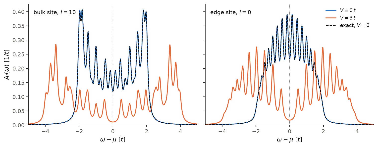
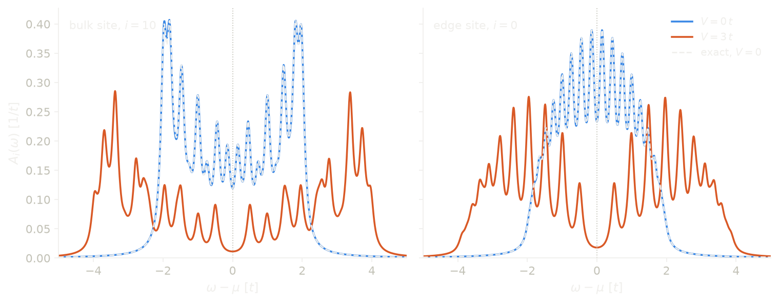
The figure shows \(A_i(\omega)\) of an open chain of 20 spinless fermions at
half filling, with
\(H=-t\sum_i(c^\dagger_ic_{i+1}+\mathrm{h.c.})+V\sum_i(n_i-\frac12)(n_{i+1}-\frac12)\),
from get_spectral_function with nex=50 and \(\delta=0.1\). The left panel
is a site in the middle of the chain and the right panel the edge site. At
\(V=0\) the result lies on the exact free-fermion spectrum (dashed): 20
levels inside the band \(|\omega|<2t\), with a weight that depends on the
site. In the middle of the chain the weight piles up at the band edges, as
in \(1/\sqrt{4t^2-\omega^2}\). At the edge it is largest at the band center.
At \(V=3t\) the chain is a charge density wave, and a gap of about \(t\) opens
at \(\omega=\mu\). The weight moves to higher energies, around \(\pm V\). Here
the 50 states hold 79 per cent of the weight at the middle site, so part of
the spectrum at high energy is missing; info["particle"]["captured"] and
info["hole"]["captured"] tell this.
Code of this figure (docs/figures/dynamical-correlators_ldos/)
# Local density of states A_i(omega) of a half-filled open chain of spinless
# fermions, at a bulk site and at the edge, for V=0 and V=3t (charge density
# wave), with the exact free-fermion spectrum as the reference at V=0.
import numpy as np
from dmrgpy import fermionchain

n = 20
N = n//2  # half filling
Vs = [0.0, 3.0]
sites = [n//2, 0]
nex, delta = 50, 0.1
es = np.linspace(-5.0, 5.0, 1000)

# free fermions on the same open chain, Lorentzian broadening delta
eps, phi = np.linalg.eigh(-(np.eye(n, k=1) + np.eye(n, k=-1)))
mu_free = (eps[N-1] + eps[N])/2
A_free = [sum(phi[i, k]**2*delta/np.pi/((es - eps[k] + mu_free)**2 + delta**2)
              for k in range(n)) for i in sites]

A, captured, gap = [], [], []
for V in Vs:
    fc = fermionchain.Fermionic_Chain(n)
    h = sum(-fc.Cdag[i]*fc.C[i+1] - fc.Cdag[i+1]*fc.C[i]
            + V*(fc.N[i] - 0.5)*(fc.N[i+1] - 0.5) for i in range(n-1))
    fc.set_hamiltonian(h)
    fc.maxm, fc.nsweeps, fc.cutoff = 80, 12, 1e-12
    fc.set_conserved_sector(Nf=N)
    for i in sites:  # the same chain, so the sector states are reused
        _, a, info = fc.get_spectral_function(i=i, nex=nex, es=es, delta=delta,
                                              return_poles=True)
        A.append(np.real(a))
        captured.append([info["particle"]["captured"], info["hole"]["captured"]])
    gap.append(info["gap"])

np.savez("data.npz", Vs=Vs, sites=sites, es=es,
         A=np.reshape(A, (len(Vs), len(sites), len(es))),
         captured=np.reshape(captured, (len(Vs), len(sites), 2)),
         gap=gap, A_free=A_free)
import numpy as np
import style

d = np.load("data.npz")
es, A, A_free, Vs, sites = d["es"], d["A"], d["A_free"], d["Vs"], d["sites"]


def draw(theme):
    c = style.colors(theme)
    fig, axs = style.figure(2, sharey=True)
    for j, (ax, i) in enumerate(zip(axs, sites)):
        for k, V in enumerate(Vs):
            ax.plot(es, A[k, j], color=c["series"][k], lw=style.LW,
                    label=r"$V=%g\,t$" % V)
        ax.plot(es, A_free[j], **style.reference(theme), label="exact, $V=0$")
        ax.axvline(0.0, color=c["ink2"], lw=0.8, ls=":")
        ax.set_xlim(es[0], es[-1])
        ax.set_ylim(0, None)
        ax.set_xlabel(r"$\omega-\mu$ [$t$]")
        where = "bulk" if i > 0 else "edge"
        ax.text(0.03, 0.95, "%s site, $i=%d$" % (where, i),
                transform=ax.transAxes, va="top", color=c["ink"])
    axs[0].set_ylabel(r"$A_i(\omega)$ [$1/t$]")
    axs[1].legend(loc="upper right")
    fig.tight_layout()
    return fig


style.main(draw, "dynamical-correlators_ldos")
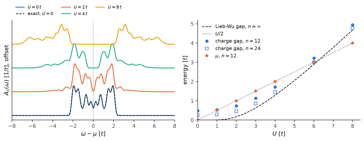
The left panel shows \(A_{ii}(\omega)\) at a bulk site of a half-filled Hubbard chain with \(n=12\), from the two KPM correlators above with \(\delta=0.25\). We write the interaction as \(U\sum_i(n_{i\uparrow}-\frac12)(n_{i\downarrow}-\frac12)\), so the global ground state is at half filling and \(\mu=0\). At \(U=0\) the result lies on the exact free-fermion spectrum (dashed), drawn with the same KPM kernel. As \(U\) grows, the single band splits into a lower and an upper Hubbard band. The right panel shows the charge gap from the ground states of the sectors \(N-1\), \(N\) and \(N+1\). It approaches the Lieb-Wu gap of the infinite chain (dashed) as \(n\) grows, and the finite chains stay above it because of the level spacing. For these sectors we use \(U\sum_in_{i\uparrow}n_{i\downarrow}\), and the chemical potential comes out exactly at \(U/2\), as particle-hole symmetry requires.
Code of this figure (docs/figures/dynamical-correlators_spectral_function/)
# Mott gap of the half-filled Hubbard chain. Local spectral function A_ii(w)
# of a bulk site (spin up) from KPM, and the charge gap from the ground
# states of the sectors N-1, N, N+1, against the Lieb-Wu gap.
import numpy as np
from scipy.integrate import quad
from dmrgpy import fermionchain, kpmdmrg

n = 12
site = n//2
Us_spec = [0.0, 2.0, 4.0, 8.0]
Us_gap = [0.0, 1.0, 2.0, 3.0, 4.0, 6.0, 8.0]
ns_gap = [n, 2*n]
delta = 0.25
es = np.linspace(-8.0, 8.0, 800)


def hubbard(U, n, shifted):
    # shifted: U (n_up-1/2)(n_dn-1/2), particle-hole symmetric, so mu=0
    fc = fermionchain.Spinful_Fermionic_Chain_Native(n)
    h = sum(-cd[i]*c[i+1] - cd[i+1]*c[i] for i in range(n-1)
            for cd, c in ((fc.Cdagup, fc.Cup), (fc.Cdagdn, fc.Cdn)))
    if shifted:
        h = h + sum(U*(fc.Nup[i] - 0.5)*(fc.Ndn[i] - 0.5) for i in range(n))
    else:
        h = h + sum(U*fc.Nup[i]*fc.Ndn[i] for i in range(n))
    fc.set_hamiltonian(h)
    fc.maxm, fc.nsweeps, fc.cutoff, fc.kpmmaxm = 80, 12, 1e-12, 80
    return fc


def kpm(fc, A, B):
    # KPM moments of (A,B) with the rescaling needed to rebuild a spectrum
    mus, emin, emax, scale, npol, d = fc.get_dynamical_correlator_moments(
        name=(A, B), delta=delta)
    return dict(mus=np.asarray(mus), emin=emin, emax=emax, scale=scale,
                npol=npol, d=d, e0=fc.e0)


def spectrum(x, m):
    return kpmdmrg.dynamical_correlator_from_moments(
        m["mus"], m["emin"], m["emax"], m["scale"], m["npol"], x,
        kernel="jackson", delta=m["d"], origin=m["e0"])[1].real


def exact(m, poles, weights):
    # m with its moments replaced by the exact ones of a set of poles
    x = (poles + m["e0"] - (m["emin"] + m["emax"])/2)*m["scale"]
    j = np.arange(len(m["mus"]))[:, None]
    return dict(m, mus=np.sum(weights*np.cos(j*np.arccos(x)), axis=1))


# free fermions at the site: levels, weights, empty levels at half filling
eps, phi = np.linalg.eigh(-(np.eye(n, k=1) + np.eye(n, k=-1)))
w, empty = phi[site]**2, eps > 0

A = []
for U in Us_spec:
    fc = hubbard(U, n, shifted=True)
    fc.gs_energy()
    mp = kpm(fc, fc.Cup[site], fc.Cdagup[site])  # addition, w > 0
    mh = kpm(fc, fc.Cdagup[site], fc.Cup[site])  # removal, w < 0
    A.append(spectrum(es, mp) + spectrum(-es, mh))
    if U == 0.0:  # exact free-fermion moments, same rescaling and kernel
        A_free = (spectrum(es, exact(mp, eps[empty], w[empty]))
                  + spectrum(-es, exact(mh, -eps[~empty], w[~empty])))

# charge gap and mu from the sectors N-1, N, N+1, with U n_up n_dn
gap, mu = np.zeros((2, len(ns_gap), len(Us_gap)))
for a, L in enumerate(ns_gap):
    for b, U in enumerate(Us_gap):
        e = []
        for dN in (-1, 0, 1):
            fc = hubbard(U, L, shifted=False)
            fc.set_conserved_sector(Nf=L + dN, Sz=dN)
            e.append(fc.gs_energy())
        gap[a, b], mu[a, b] = e[0] + e[2] - 2*e[1], (e[2] - e[0])/2


def lieb_wu(U):
    # charge gap of the infinite chain, t=1
    f = lambda y: np.sqrt(y*y - 1)/np.sinh(min(2*np.pi*y/U, 700.0))
    return 16/U*quad(f, 1, np.inf, limit=400)[0] if U > 0 else 0.0


Ul = np.linspace(0, max(Us_gap), 200)
np.savez("data.npz", Us_spec=Us_spec, es=es, A=A, A_free=A_free,
         Us_gap=Us_gap, ns_gap=ns_gap, gap=gap, mu=mu,
         Ul=Ul, gap_lw=[lieb_wu(U) for U in Ul])
import numpy as np
import style

d = np.load("data.npz")
es, A, Us = d["es"], d["A"], d["Us_spec"]
off = 0.8*np.max(A)  # vertical offset between the spectra


def draw(theme):
    c = style.colors(theme)
    fig, (a1, a2) = style.figure(2)
    for k, u in enumerate(Us):
        a1.plot(es, A[k] + k*off, color=c["series"][k], lw=style.LW,
                label=r"$U=%g\,t$" % u)
        if k == 0:
            a1.plot(es, d["A_free"], **style.reference(theme),
                    label="exact, $U=0$")
    a1.axvline(0.0, color=c["ink2"], lw=0.8, ls=":")
    a1.set_xlim(es[0], es[-1])
    a1.set_yticks([])
    a1.set_xlabel(r"$\omega-\mu$ [$t$]")
    a1.set_ylabel(r"$A_{ii}(\omega)$ [$1/t$], offset")
    a1.legend(loc="lower left", bbox_to_anchor=(0.0, 1.0), ncol=3, fontsize=8)

    a2.plot(d["Ul"], d["gap_lw"], **style.reference(theme),
            label="Lieb-Wu gap, $n=\\infty$")
    a2.plot(d["Ul"], d["Ul"]/2, color=c["ink2"], ls=":", lw=style.LW_REF,
            label=r"$U/2$")
    for k, (L, m) in enumerate(zip(d["ns_gap"], "os")):
        a2.plot(d["Us_gap"], d["gap"][k], m, color=c["series"][0],
                mfc="none" if k else c["series"][0],
                label="charge gap, $n=%d$" % L)
    a2.plot(d["Us_gap"], d["mu"][0], "D", color=c["series"][1], ms=4,
            label=r"$\mu$, $n=%d$" % d["ns_gap"][0])
    a2.set_xlabel(r"$U$ [$t$]")
    a2.set_ylabel(r"energy [$t$]")
    a2.set_xlim(0, None)
    a2.set_ylim(0, None)
    a2.legend(loc="upper left")
    fig.tight_layout()
    return fig


style.main(draw, "dynamical-correlators_spectral_function")
Any pair of operators
name=(A, B) accepts any operators built from the chain operators, for
example a bond operator:
A = hc.Cdagup[0]*hc.Cup[1]
(x, y) = hc.get_dynamical_correlator(name=(A, A.get_dagger()), es=es, delta=0.1)
The pair may also be operators already converted with sc.toMPO(A)
(Hamiltonians and operators). This avoids building them again in a scan over parameters. It works
with the DMRG submodes "EX", "CVM" and "ROOTN", and with
mode="ED" when the operators are built with sc.toMPO(A, mode="ED").
The other submodes raise an error and need the operator itself.