Fidelity susceptibility
Let the Hamiltonian depend on a parameter, \(H(\lambda)=H_0+\lambda H_1\). The fidelity susceptibility measures how fast the ground state changes with \(\lambda\). In perturbation theory it is
At a quantum phase transition the gap closes and \(\chi\) has a peak that
grows with system size. So a scan of \(\chi(\lambda)\) locates a critical
point without knowing the order parameter. Here sc is a spin chain:
from dmrgpy import fidelity
h0 = 4*sum(sc.Sz[i]*sc.Sz[i+1] for i in range(n-1))   # Ising coupling
h1 = 2*sum(sc.Sx[i] for i in range(n))                # transverse field
chi = fidelity.get_fidelity(sc, h0, h1, 1.0)               # default
chi_pt = fidelity.get_fidelity(sc, h0, h1, 1.0, fmode="PT")  # formula above
The default, fmode="derivative", does not use the formula above. It
computes the second derivative of the ground-state overlap by finite
differences, so it needs only ground states. If the ground state is
degenerate within delta, it uses the overlap matrix of the degenerate
states and returns the sum of \(\chi\) over these states. fmode="PT" sums
over the n lowest states. Increase n
until \(\chi\) stops changing. The keywords are:
dl: the finite-difference step in \(\lambda\) (default 0.1). Use a smaller value when \(\chi\) changes fast.n,delta: for the default estimator, the number of low states searched for a degenerate ground state, and the energy tolerance for calling two states degenerate. Forfmode="PT",nis the number of states in the sum (default 2) anddeltais the \(\delta\) of the formula above.mode="ED": exact diagonalization, for small chains.
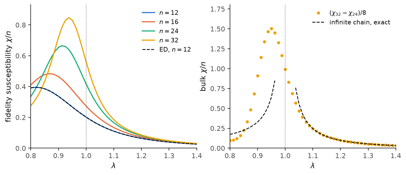
The figure shows open Ising chains, \(H=\sum_i\sigma^z_i\sigma^z_{i+1}+\lambda\sum_i\sigma^x_i\),
computed with dl=0.02. On the left is \(\chi/n\) for four lengths. The
peak grows with \(n\) and moves towards the critical point \(\lambda=1\): it
is at \(\lambda=0.83\), 0.86, 0.91 and 0.94 for \(n=12\), 16, 24 and 32. For
\(n=12\) the ED curve (dashed line) covers the DMRG one. On the right, the
difference of the two longest chains removes the contribution of the
edges and gives \(\chi/n\) of the bulk. From about \(\lambda=1.1\) it lies on the
exact result of the infinite chain, \(1/[16\lambda^2(\lambda^2-1)]\). On the
ordered side the exact result is \(1/[16(1-\lambda^2)]\), and the two chains
are still too short to reach it: the difference crosses it at
\(\lambda=0.85\) and lies below it at \(\lambda=0.8\). The exact free-fermion
solution of the open chain shows that at \(\lambda=0.8\) the difference
reaches the bulk value only for \(n\) of about 50. Close to \(\lambda=1\) the correlation length is longer than
the chains, so they do not reach the infinite-chain result there.
We start the scan at \(\lambda=0.8\). In the ordered phase the two lowest
states of an open chain have an energy splitting that decays with \(n\).
For \(n=32\) it is \(6\times10^{-4}\) at \(\lambda=0.8\) and drops below the
default delta near \(\lambda=0.75\). Below that point the default
estimator returns \(\chi\) summed over the two states. A smaller delta
does not help: DMRG does not separate two states this close in energy,
and the overlaps are then not meaningful.
Code of this figure (docs/figures/fidelity_ising/)
# Fidelity susceptibility of the open transverse-field Ising chain
# H = sum sz_i sz_i+1 + lambda sum sx_i (Pauli matrices) across lambda = 1,
# with ED on the shortest chain as the reference.
import numpy as np
from dmrgpy import spinchain, fidelity

ns = [12, 16, 24, 32]
# lambda starts at 0.8: below about 0.75 the Z2 doublet of the ordered
# chain splits by less than tol at n=32, and chi mixes the two states
lams = np.round(np.linspace(0.8, 1.4, 49), 8)
dl, tol = 0.02, 1e-4


def chain(n):
    sc = spinchain.Spin_Chain(["S=1/2"]*n)
    sc.maxm, sc.nsweeps = 60, 20
    h0 = 4*sum(sc.Sz[i]*sc.Sz[i+1] for i in range(n-1))
    h1 = 2*sum(sc.Sx[i] for i in range(n))
    sc.set_hamiltonian(h0 + h1)
    return sc, h0, h1


def chi(n, **kw):  # chi, total over the chain, at every lambda
    sc, h0, h1 = chain(n)
    return [fidelity.get_fidelity(sc, h0, h1, l, dl=dl, delta=tol,
                                  fmode="derivative", **kw) for l in lams]


chi_dmrg = [chi(n) for n in ns]
chi_ed = chi(ns[0], mode="ED")

np.savez("data.npz", lam=lams, ns=ns, chi=chi_dmrg, chi_ed=chi_ed)
import numpy as np
import style

d = np.load("data.npz")
lam, ns, chi = d["lam"], d["ns"], d["chi"]


def bulk(l):  # infinite chain, per site
    return np.where(l < 1, 1/(16*(1-l**2)), 1/(16*l**2*(l**2-1)))


# the edge contribution cancels in the difference of the two longest
# chains, which leaves the bulk value per site
n1, n2 = ns[-2], ns[-1]
dens = (chi[-1] - chi[-2])/(n2 - n1)


def draw(theme):
    c = style.colors(theme)
    fig, (a, b) = style.figure(2)
    for k, n in enumerate(ns):
        a.plot(lam, chi[k]/n, "-", color=c["series"][k], label=r"$n=%d$" % n)
    a.plot(lam, d["chi_ed"]/ns[0], **style.reference(theme),
           label=r"ED, $n=%d$" % ns[0])
    a.set_ylabel(r"fidelity susceptibility $\chi/n$")
    a.set_ylim(0, 1.1*np.max(chi[-1]/ns[-1]))
    b.plot(lam, dens, "o", ms=3.5, color=c["series"][len(ns)-1],
           label=r"$(\chi_{%d}-\chi_{%d})/%d$" % (n2, n1, n2 - n1))
    for k, side in enumerate((lam < 0.97, lam > 1.03)):
        b.plot(lam[side], bulk(lam[side]), **style.reference(theme),
               label="infinite chain, exact" if k == 0 else None)
    b.set_ylabel(r"bulk $\chi/n$")
    b.set_ylim(0, 1.2*np.max(dens))
    for ax in (a, b):
        ax.axvline(1.0, color=c["ink2"], lw=0.8, ls=":")
        ax.set_xlabel(r"$\lambda$")
        ax.set_xlim(lam[0], lam[-1])
        ax.legend(loc="upper right")
    return fig


style.main(draw, "fidelity_ising")