Mean-field decoupling
For a spin Hamiltonian with exchange couplings \(J_{ij}\), the self-consistent mean-field (Weiss-field) decoupling replaces the exchange by a field on each site,
We solve \(H_{\rm MF}\), compute the new \(\langle\mathbf S_i\rangle\), rebuild
\(\mathbf h_i\), mix the old and new values, and repeat until the
magnetization stops changing. With \(p=0\) this is pure mean-field theory.
With \(0<p<1\) a fraction \(p\) of the exchange is kept and treated exactly,
together with the field. With \(p=1\) it is the original model. The
couplings are read from the Hamiltonian of the chain, so any one- and
two-site spin Hamiltonian works, including anisotropic and long-range
exchange. Here sc is the Heisenberg chain of Ground state:
from dmrgpy import meanfield
n = sc.ns
m0 = [[0, 0, 0.5*(-1)**i] for i in range(n)]       # staggered start
mf = meanfield.spinchain_meanfield(sc, p=0.0, m0=m0, mix=0.5)
m = mf.get_magnetization()       # self-consistent <S_i>, a 3 x n array
e = mf.gs_energy()               # mean-field energy
The function returns a new chain whose Hamiltonian is the converged
\(H_{\rm MF}\). This Hamiltonian includes the constant
\(-(1-p)\sum_{ij}J_{ij}\langle\mathbf S_i\rangle\cdot\langle\mathbf S_j\rangle\),
so the exchange is not counted twice. At \(p=0\) its gs_energy() is the
expectation value of the original Hamiltonian in the mean-field state.
The keywords are:
p: the fraction of the exchange kept exactly.m0: the starting magnetization, one 3-vector per site. Random by default. For an antiferromagnet start from a staggered pattern, since simple mixing can oscillate otherwise.mix: the weight of the new magnetization in each step (default 0.9). Lower it if the loop oscillates.maxerror,maxite: the convergence tolerance and the maximal number of iterations. Aftermaxitethe loop stops with a warning.mixmode:"default"(linear mixing) or"broyden".mode="ED": solve each step with exact diagonalization.
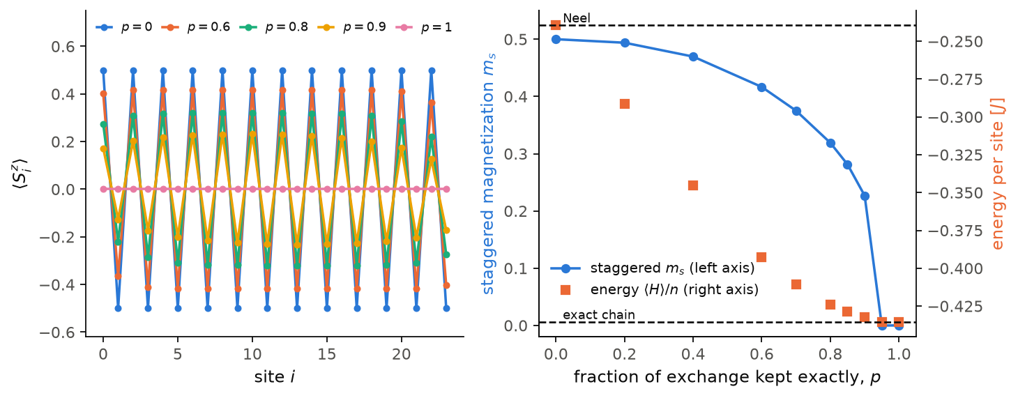
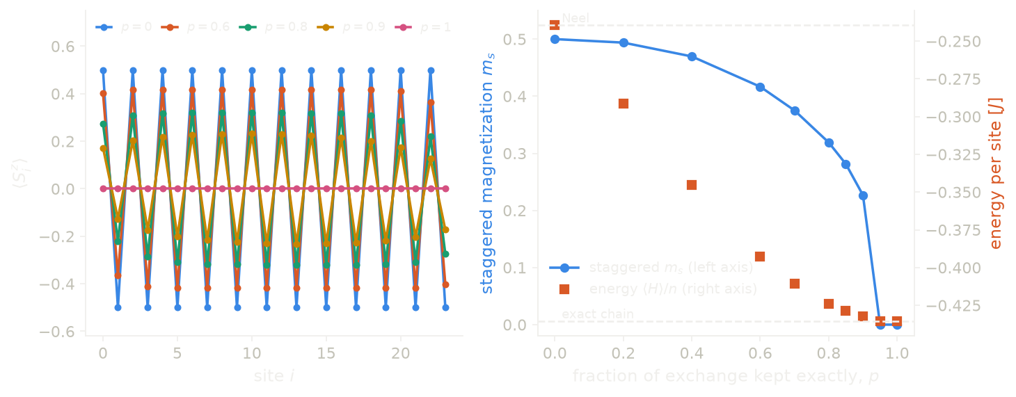
The figure shows the Heisenberg chain with \(n=24\) sites, started from the
staggered pattern above. On the left is \(\langle S^z_i\rangle\). At \(p=0\)
it is the classical Neel state with \(|\langle S^z_i\rangle|=1/2\). As \(p\)
grows, the order gets weaker. On the right, the staggered magnetization
of the 12 central sites falls with \(p\) and drops to zero between \(p=0.9\)
and \(p=0.95\), before \(p=1\): in a finite chain the order disappears once
the Weiss field is small compared with the finite-size gap. The squares
are \(\langle H\rangle\) of the original Heisenberg chain in the
self-consistent state, not gs_energy() of the returned chain, which
differs from it for \(0<p<1\). The energy goes from the Neel value
\(-(n-1)/(4n)\) at \(p=0\) to the exact energy of the chain at \(p=1\). In the
bulk this exact energy is \(1/4-\log2=-0.443\) per site; the open chain
with \(n=24\) gives \(-0.4356\), because of its edges.
Code of this figure (docs/figures/mean-field_neel/)
# Self-consistent mean-field decoupling of the spin-1/2 Heisenberg chain, as
# the fraction p of the exchange kept exactly goes from 0 (pure mean field)
# to 1 (the exact chain), started from a Neel state.
import numpy as np
from dmrgpy import spinchain, meanfield

n = 24
ps = [0, 0.2, 0.4, 0.6, 0.7, 0.8, 0.85, 0.9, 0.95, 1.0]

sc = spinchain.Spin_Chain(["S=1/2"]*n)
sc.maxm, sc.nsweeps = 60, 12
h = sum(sc.Sx[i]*sc.Sx[i+1] + sc.Sy[i]*sc.Sy[i+1] + sc.Sz[i]*sc.Sz[i+1]
        for i in range(n-1))
sc.set_hamiltonian(h)
e_exact = sc.gs_energy()

m0 = [[0, 0, 0.5*(-1)**i] for i in range(n)]  # staggered initial guess
mz, e_var, e_mf = [], [], []
for p in ps:
    mf = meanfield.spinchain_meanfield(sc, p=p, m0=m0, mix=0.5,
                                       maxerror=1e-6, maxite=500)
    mz.append(np.real(mf.get_magnetization())[2])  # <Sz_i>
    e_var.append(mf.vev(h).real)  # <H> of the original chain
    e_mf.append(mf.gs_energy())   # energy of the mean-field chain itself

np.savez("data.npz", n=n, p=ps, mz=mz, e_var=e_var, e_mf=e_mf,
         e_exact=e_exact)
import numpy as np
import style

d = np.load("data.npz")
n, p, mz = int(d["n"]), d["p"], d["mz"]
e_neel, e_exact = -(n-1)/(4*n), float(d["e_exact"])/n
# staggered magnetization of the 12 central sites
centre = np.arange((n - 12)//2, (n + 12)//2)
ms = np.mean((-1.0)**centre*mz[:, centre], axis=1)
show = [0.0, 0.6, 0.8, 0.9, 1.0]


def draw(theme):
    c = style.colors(theme)
    fig, (a, b) = style.figure(2)
    shown = [j for j, pj in enumerate(p)
             if np.min(np.abs(pj - np.array(show))) < 1e-9]
    for k, j in enumerate(shown):
        a.plot(np.arange(n), mz[j], "o-", ms=3.5, color=c["series"][k],
               label=r"$p=%g$" % p[j])
    a.set_xlabel(r"site $i$")
    a.set_ylabel(r"$\langle S^z_i\rangle$")
    a.set_ylim(-0.62, 0.75)
    a.legend(loc="upper center", ncol=5, fontsize=8, handlelength=1.2,
             columnspacing=0.8)

    b.plot(p, ms, "o-", color=c["series"][0],
           label=r"staggered $m_s$ (left axis)")
    b.set_xlabel(r"fraction of exchange kept exactly, $p$")
    b.set_ylabel(r"staggered magnetization $m_s$", color=c["series"][0])
    b.set_ylim(-0.02, 0.55)
    b2 = b.twinx()
    b2.spines["right"].set_visible(True)
    b2.spines["top"].set_visible(False)
    b2.plot(p, d["e_var"]/n, "s", color=c["series"][1],
            label=r"energy $\langle H\rangle/n$ (right axis)")
    for e, name in ((e_neel, "Neel"), (e_exact, "exact chain")):
        b2.axhline(e, **style.reference(theme))
        b2.text(0.02, e, name, va="bottom", fontsize=8, color=c["ink"])
    b2.set_ylabel(r"energy per site [$J$]", color=c["series"][1])
    h1, l1 = b.get_legend_handles_labels()
    h2, l2 = b2.get_legend_handles_labels()
    b.legend(h1 + h2, l1 + l2, loc="lower left", bbox_to_anchor=(0.0, 0.08))
    return fig


style.main(draw, "mean-field_neel")
meanfield.decompose_spin_hamiltonian(sc) returns the onsite fields
b[i,a], the exchange J[i,j,a,b] and the constant read from the
Hamiltonian. A Hamiltonian that is not of this form, for example with a
three-site term, raises an error.